See also
A Jupyter notebook version of this tutorial can be downloaded here.
Acquisitions#
Introduction#
This tutorial provides examples of how to add acquisitions to schedules and retrieve the corresponding results.
The fundamental data structure returned by an acquisition is an xarray.Dataset (official documentation), which consists of multiple xarray.DataArray.
Initial setup#
First, we set up the connection to the cluster and hardware configuration.
The introduction and parametrization of a qubit is not mandatory for running acquisitions. Hence schedules presented in this tutorial will remain at the pulse-level description.
[1]:
from typing import Any

import xarray

from qblox_scheduler import HardwareAgent
/.venv/lib/python3.14/site-packages/quantify_core/visualization/instrument_monitor.py:13: QCoDeSDeprecationWarning: The `qcodes.utils.helpers` module is deprecated. Please consult the api documentation at https://microsoft.github.io/Qcodes/api/index.html for alternatives.
  from qcodes.utils.helpers import strip_attrs
[2]:
hardware_config: dict[str, Any] = {
    "version": "0.2",
    "config_type": "QbloxHardwareCompilationConfig",
    "hardware_description": {
        "cluster0": {
            "instrument_type": "Cluster",
            "modules": {"4": {"instrument_type": "QRM"}},
            "ref": "internal",
        }
    },
    "hardware_options": {},
    "connectivity": {
        "graph": [
            ["cluster0.module4.complex_output_0", "q0:port"],
            ["cluster0.module4.complex_input_0", "q0:port"],
        ]
    },
}

hardware_agent: HardwareAgent = HardwareAgent(hardware_configuration=hardware_config)
hardware_agent.connect_clusters()
# note: if the call to the connect_cluster method is dropped, it would happen anyway automatically at the next call to
#       a run method. Using connect_cluster explicitly is therefore not mandatory.
/.venv/lib/python3.14/site-packages/qblox_scheduler/qblox/hardware_agent.py:556: UserWarning: cluster0: Trying to instantiate cluster with ip 'None'.Creating a dummy cluster.
  warnings.warn(
Pulse-level acquisitions#
Pulse-level acquisitions define when and how to store and retrieve input signals coming from the device. They are described by their timing information (start time and length), protocol, acq_channel and coordinates.
Timing information specifies when the acquisition happens on the schedule.
Protocol defines which hardware or software formatting is done on the input signal.
acq_channelandcoordstogether identify acquisitions and data points for the user in the returned dataset:acq_channelidentifies a particularDataArray, while every point within such an array is identified by coordinates.
In the following subsections we give examples for each supported acquisition protocol.
We assume, that these tutorials are run on a Qblox QRM module. On the QRM module \(\text{O}^{[1]}\) is connected to \(\text{I}^{[1]}\) and \(\text{O}^{[2]}\) is connected to \(\text{I}^{[2]}\).
The physical length of the cables connecting output to input channels introduces a delay before a sent signal is received. This delay is known as the TIME_OF_FLIGHT.
Trace acquisition#
One of the simplest protocols is the trace (or scope) acquisition. With this protocol, one can acquire the time trace of a waveform, just like with an oscilloscope. The sampling rate is 1GSa/s, and the maximum duration of a single Trace acquisition is 16us. In this subsection we will send out a DRAG pulse on the output, then measure it with the input of the QRM, and plot the retrieved data.
Setting up the schedule#
The schedule is straightforward: it emits a pulse on an output port and then initiates a trace acquisition on the corresponding input port, delayed by TIME_OF_FLIGHT to account for the signal travel time.
We choose to play a DRAG pulse, whose duration is defined using the parameter PULSE_DURATION. We define a separate parameter ACQ_DURATION, allowing the acquisition duration to be larger than the duration of the pulse (e.g., in case the TIME_OF_FLIGHT was not yet calibrated).
[3]:
# parameters for the experiment
# --------------------------------
TIME_OF_FLIGHT: float = 148e-9
PULSE_DURATION: float = 1e-6
PULSE_AMPLITUDE: float = 0.1
BETA: float = 50e-9
PHASE: float = 0
ACQ_DURATION = PULSE_DURATION

from qblox_scheduler import Schedule
from qblox_scheduler.operations import DRAGPulse, IdlePulse, Trace

schedule: Schedule = Schedule("trace_acquisition_tutorial")
schedule.add(IdlePulse(duration=1e-6))

schedule.add(
    DRAGPulse(
        amplitude=PULSE_AMPLITUDE,
        beta=BETA,
        duration=PULSE_DURATION,
        phase=PHASE,
        port="q0:port",
        clock="cl0.baseband",
    ),
)
schedule.add(
    Trace(duration=ACQ_DURATION, port="q0:port", clock="cl0.baseband"),
    ref_pt="start",
    rel_time=TIME_OF_FLIGHT,
)

xr_trace_acquisition: xarray.Dataset = hardware_agent.run(schedule)
[4]:
import numpy as np

from qblox_scheduler.waveforms import drag


def drag_pulse_waveform():
    t = np.arange(0, PULSE_DURATION, 1e-9)
    wave = drag(t=t, amplitude=PULSE_AMPLITUDE, beta=BETA, duration=PULSE_DURATION, nr_sigma=4)

    return wave


xr_trace_acquisition[0].data = [drag_pulse_waveform()]
Compile and run the schedule, retrieving acquisition#
As you may have already noticed, acquisitions are directly returned by the run method of the HardwareAgent. The returned data is an xarray.Dataset:
[5]:
xr_trace_acquisition
[5]:
<xarray.Dataset> Size: 24kB
Dimensions:        (trace_index_0: 1000, acq_index_0: 1)
Coordinates:
  * trace_index_0  (trace_index_0) int64 8kB 0 1 2 3 4 5 ... 995 996 997 998 999
  * acq_index_0    (acq_index_0) int64 8B 0
Data variables:
    0              (acq_index_0, trace_index_0) complex128 16kB (-5.448662043...
Attributes:
tuid: 20260710-175608-433-191d0aIf we pay attention to the content and structure of this Dataset, we can already notice some important features:
The acquired data are stored in a “Data variables” mapping. For each acquisition channel, there is a corresponding
xarray.DataArrayin this mapping. Theqblox-scheduleracquisition operations (Tracein above example) have anacq_channeloptional argument: for each acquisition channel declared, a new data variable in the resultingxarray.Datasetis created, and the correspondingxarray.DataArrayof measures is attached to it. In this example, we omitted theacq_channelargument, so the scheduler assigned the default channel name, 0.Each
xarray.DataArraycontains the measured data series, whose values are labeled using a coordinate system. By default, aacq_index_<acq_channel>coordinate axis –corresponding to the integer indexing of the acquisitions– is always created, but other coordinates can be defined by the user, more details about it will be given later in this tutorial.
In our case, with a Trace acquisition, each acq_index_<acq_channel> value represents a 1ns long measurement, which is the time resolution of the sequencers implemented on Qblox modules. The real and imaginary parts of the data correspond to the I and Q components, respectively.
xarray.Datasets embeds a wrapper to the matplotlib plotting library. We can use it to quickly visualize the acquired data:
[6]:
import matplotlib.pyplot as plt

fig, axs = plt.subplots(1)

xr_trace_acquisition[0].real.plot(ax=axs, label="I")
xr_trace_acquisition[0].imag.plot(ax=axs, label="Q")

axs.set_title("")
axs.set_ylabel("")
axs.legend()
plt.show()
Single-sideband integration acquisition#
The single-sideband integration protocol involves integrating the complex input signal over a given time period. The integration weight is a square window (this window’s length is the acquisition duration). The signal is demodulated with an using the specified clock before the integration happens, enabling experiments based on heterodyne detection.
In this tutorial, we will send 4 square pulses out, and measure it in 4 separate bins. Acquisitions will be grouped in two channels: acquisitions assigned to the same channel are appended one after another, and populate new bins. We will also send out purely real and imaginary pulses (or purely I and purely Q pulses), and observe that they appear as real and imaginary acquisitions. In the case of single-sideband integration the integration happens after demodulation.
You can use different acquisition channels to distinguish between measurements on different qubits or to separate data from successive experiments on the same qubit. In our simple example, we only use a single port-clock combination for both acquisition channels, we will then verify that those acquisition channels are reported as different data variables of a same returned xarray.Dataset.
Setting up the schedule#
[7]:
# parameters for the experiment
# --------------------------------
TIME_OF_FLIGHT: float = 148e-9
PULSE_DURATION: float = 120e-9
ACQ_DURATION = PULSE_DURATION
We define a simple helper function that sends out the square pulse with pulse_level complex amplitude, and then measures it after TIME_OF_FLIGHT seconds.
[8]:
from qblox_scheduler import Schedule
from qblox_scheduler.operations import IdlePulse, SquarePulse, SSBIntegrationComplex

schedule: Schedule = Schedule("ssb_acquisition_tutorial")


def pulse_and_acquisition(pulse_level, acq_channel, schedule) -> None:
    schedule.add(
        SquarePulse(
            duration=PULSE_DURATION,
            amplitude=pulse_level,
            port="q0:port",
            clock="cl0.baseband",
        ),
        ref_pt="end",
        rel_time=1e-6,  # Idle time before the pulse is played
    )
    schedule.add(
        SSBIntegrationComplex(
            duration=ACQ_DURATION,
            port="q0:port",
            clock="cl0.baseband",
            acq_channel=acq_channel,
        ),
        ref_pt="start",
        rel_time=TIME_OF_FLIGHT,
    )


pulse_and_acquisition(pulse_level=0.5, acq_channel="ch0", schedule=schedule)
pulse_and_acquisition(pulse_level=0.5j, acq_channel="ch0", schedule=schedule)
pulse_and_acquisition(pulse_level=1, acq_channel="ch1", schedule=schedule)
pulse_and_acquisition(pulse_level=1j, acq_channel="ch1", schedule=schedule)
Running the schedule, retrieving acquisition#
Acquisitions are directly returned by the run method of the HardwareAgent.
[9]:
xr_ssb_acquisition: xarray.Dataset = hardware_agent.run(schedule)
[10]:
import xarray as xr

xr_ssb_acquisition = xr.open_dataset("./utils/data/data_simple_ssb.hdf5", engine="h5netcdf")
xr_ssb_acquisition["ch0"].data
xr_ssb_acquisition["ch1"].data
[10]:
array([0.5321534-0.01356424j, 0.0178002+0.49121983j])
[11]:
xr_ssb_acquisition
[11]:
<xarray.Dataset> Size: 96B
Dimensions:        (acq_index_ch0: 2, acq_index_ch1: 2)
Coordinates:
  * acq_index_ch0  (acq_index_ch0) int64 16B 0 1
  * acq_index_ch1  (acq_index_ch1) int64 16B 0 1
Data variables:
    ch0            (acq_index_ch0) complex128 32B (0.2759775280898876-0.01315...
    ch1            (acq_index_ch1) complex128 32B (0.5321533952125062-0.01356...
Attributes:
tuid: 20250922-155050-277-2c85f4There are now two xarray.DataArrays in this xarray.Dataset. These correspond to acq_channel="ch0" and acq_channel="ch1".
As expected, the single side band integration produced four complex numbers: for each acquisition channel, SSBIntegrationComplex integrates the successively acquired values. One purely real value in acq_index_<acq_channel>=0 and one purely imaginary value in acq_index_<acq_channel>=1. Notice, that the amplitude is double in the case of acq_channel="ch1" compared to acq_channel="ch0".
Acquisition coordinates#
General concept#
qblox-scheduler uses the concept of acquisition coordinates to link measurement data directly to the physical parameters being swept in a schedule. When an experiment involves swept parameters (e.g. a pulse amplitude or a clock frequency), these parameters can be assigned as coordinates to the corresponding acquisitions. This provides a natural and convenient way to structure the resulting data.
To illustrate this feature, let’s have a look to the following schedule, performing a two-dimension sweep over a pulse amplitude and frequency:
[12]:
# parameters for the experiment
# --------------------------------
START_FREQ: float = 80e6
STOP_FREQ: float = 82.5e6
NUM_FREQ: int = 100
START_AMP: float = -1.0
STOP_AMP: float = 1.0
NUM_AMPS: int = 10
TIME_OF_FLIGHT: float = 148e-9
[13]:
from qblox_scheduler import ClockResource, Schedule
from qblox_scheduler.operations import (
    DRAGPulse,
    IdlePulse,
    SetClockFrequency,
)
from qblox_scheduler.operations.expressions import DType
from qblox_scheduler.operations.loop_domains import linspace

schedule: Schedule = Schedule(name="acquisition_with_coordinates_tutorial")
schedule.add_resource(ClockResource(name="clock", freq=0.0))

# nested loops over amplitude and frequency
with (
    schedule.loop(linspace(START_AMP, STOP_AMP, NUM_AMPS, dtype=DType.AMPLITUDE)) as amp,
    schedule.loop(linspace(START_FREQ, STOP_FREQ, NUM_FREQ, dtype=DType.FREQUENCY)) as freq,
):
    schedule.add(
        SetClockFrequency(
            clock="clock",
            frequency=freq,
        )
    )
    schedule.add(
        DRAGPulse(
            amplitude=amp,
            beta=0.5e-9,
            phase=0.0,
            duration=200.0e-9,
            port="q0:port",
            clock="clock",
        ),
    )
    schedule.add(
        SSBIntegrationComplex(
            port="q0:port",
            clock="clock",
            duration=100.0e-9,
            coords={
                "frequency": freq,
                "amplitude": amp,
            },  # <-- IMPORTANT: references to loop variables
            acq_channel="data",
        ),
        ref_pt="start",
        rel_time=TIME_OF_FLIGHT,
    )

xr_ssb_acquisition: xarray.Dataset = hardware_agent.run(schedule)
[14]:
import xarray as xr

xr_ssb_acquisition = xr.open_dataset("./utils/data/2d_dataset_example.hdf5", engine="h5netcdf")
Executing this schedule returned a xarray.Dataset, in which we find:
a data variable “
data” – set by theacq_channelargument ofSSBIntegrationComplex– containing the measured datathe physical coordinates
frequencyandamplitude.
The data structure reflects the parameters scanning performed during the schedule execution, making subsequent data analysis and visualization straightforward. Let’s have a look at it:
[15]:
xr_ssb_acquisition
[15]:
<xarray.Dataset> Size: 48kB
Dimensions:               (acq_index_data: 1000)
Coordinates:
  * acq_index_data        (acq_index_data) int64 8kB 0 1 2 3 ... 996 997 998 999
    amplitude             (acq_index_data) float64 8kB ...
    loop_repetition_data  (acq_index_data) int64 8kB ...
    frequency             (acq_index_data) float64 8kB ...
Data variables:
    data                  (acq_index_data) complex128 16kB ...
Attributes:
tuid: 20250911-164958-178-63babdSparse and dense representation of the data#
Looking above at how the data are formatted, one will notice that the returned data series is one dimensional (with acq_index_<acq_channel> being the dimension name). We find the coordinates amplitude and frequency in the “Coordinates” section: they also are one dimensional series, indexed by acq_index_data. Hence, acq_index_data is the unique index for all data points and additional physical coordinates of interest. It is therefore a bridge connecting those two series
families.
This representation is convenient in the general case where the dataset is “sparse” (i.e. when not all the possible tuples of coordinates values are populated by a datapoint). However, it can be simplified when the dataset is “dense” (i.e. not sparse).
To simplify the conversion of the default representation into a dense representation – where in our example the tuple of data dimension names would be (amplitude, frequency) – we provide a helper function to achieve it.
[16]:
from qblox_scheduler.analysis.helpers import acq_coords_to_dims

xr_ssb_acquisition: xarray.Dataset = acq_coords_to_dims(
    xr_ssb_acquisition, coords=["frequency", "amplitude"]
)
xr_ssb_acquisition
[16]:
<xarray.Dataset> Size: 25kB
Dimensions:               (frequency: 100, amplitude: 10)
Coordinates:
  * frequency             (frequency) float64 800B 8e+07 8.003e+07 ... 8.25e+07
  * amplitude             (amplitude) float64 80B -1.0 -0.7778 ... 0.7778 1.0
    loop_repetition_data  (frequency, amplitude) int64 8kB 0 100 200 ... 899 999
Data variables:
    data                  (frequency, amplitude) complex128 16kB (-0.05443004...
Attributes:
tuid: 20250911-164958-178-63babdThis conversion being done, we can now plot the measured data in the (I, Q) plane. To do so we will use a utility plotting function whose definition can be accessed by downloading this tutorial’s code source.
[17]:
from utils.plot_utils import plot_data_iq_plane

plot_data_iq_plane(xr_ssb_acquisition, groupby="amplitude")
The amplitude of the pulse that we measure is fixing the modulus of the data point. The frequency the pulse changes the phase of the signals at QRM input ports, hence the complex argument of the data points in the IQ plane: for a fixed value of the amplitude we observe circles in the IQ plane.
To determine the number of times you want qblox-scheduler to execute the schedule, you can set the repetitions argument or attribute for the Schedule object. By specifying a value for repetitions, you can control the number of times the schedule will run. For example, if you set repetitions to 8, the following code snippet demonstrates a schedule that would execute eight times:
schedule = Schedule(name="repeated and averaged schedule", repetitions=8)
# -----------
# OPERATIONS
#   ADDED
# ----------
schedule.add(
        SSBIntegrationComplex(
            port="port",
            clock="clock",
            duration=duration,
            acq_channel="my_measure",
        )
    )
By default, if a repetition is defined at the schedule declaration level with the Schedule(repetitions=reps) optional argument SSBIntegration operations will proceed to an averaging of the data, with respect to this global repetition loop constructed on the top of the entire schedule.
To circumvent this behavior, it possible to describe the repetition loop explicitly within the schedule itself, using a code structure like
schedule = Schedule(name="test_schedule")
with schedule.loop(arange(0, 10, 1, dtype=DType.NUMBER)) as rep:
    # -----------
    # OPERATIONS
    #   ADDED
    # ----------
    schedule.add(
            SSBIntegrationComplex(
                port="port",
                clock="clock",
                duration=duration,
                acq_channel="my_measure",
                coords={"repetitions": rep},
            )
        )
note that the repetition loop reference rep is kept as a coordinate axis of the acquisition.
Averaging during the acquisition#
This syntax for assigning coordinates to measured data series is also compatible with the description of schedules involving averaging with respect to some axes. The rule is the following: if an acquisition is nested inside a stack of loops performing parameter sweeps, any variable that is not referenced in the coords argument of the acquisition is then averaged over. It is crucial to understand, that such variable can typically be a reference to a looping operation, introduced by the python
alias keyword as, in the loop context manager. This feature is therefore made possible by the qblox-scheduler grammar for Schedules involving parameter sweeps.
Let’s take again the same illustrative example: we consider a schedule that consists of generation and acquisition of a square pulse, sweeping over the amplitude value of that pulse. For each pulse amplitude, hundred repetition cycles are run, meaning that the schedule is making use of two nested loops, for amplitude and repetition.
We will prepare two versions of that schedule, with two different version of the coords dictionary argument of the SSBIntegrationComplex: one is appending all the measures, the other is averaging over the repetitions. We set on purpose a swept amplitude range to be arbitrarily small, to see some dispersion in the acquired values for the pulse amplitudes after measuring.
[18]:
# parameters for the experiment
# --------------------------------
AMP_RANGE: float = 0.01
PULSE_DURATION: float = 200e-9
TIME_OF_FLIGHT: float = 148e-9
[19]:
from qblox_scheduler import ClockResource, Schedule
from qblox_scheduler.operations import IdlePulse, SSBIntegrationComplex
from qblox_scheduler.operations.expressions import DType
from qblox_scheduler.operations.loop_domains import arange, linspace


def schedule_builder(average_rep_axis: bool = False) -> Schedule:
    schedule: Schedule = Schedule("acquisition_averaging_tutorial")
    schedule.add_resource(ClockResource(name="clock", freq=80e6))
    schedule.add(IdlePulse(duration=1e-6))

    with (
        # Definition of the two nested loops for the amplitude sweep and the repetitions
        # and the corresponding loop variables, with the `amp` and `rep` alias references
        schedule.loop(linspace(-AMP_RANGE / 2, AMP_RANGE / 2, 21, dtype=DType.AMPLITUDE)) as amp,
        schedule.loop(arange(0, 100, 1, dtype=DType.NUMBER)) as rep,
    ):
        # depending on the `average_rep_axis` mode we select, we either keep or not the `rep` variable as a
        # coordinate of the acquisition
        coords = {"amplitude": amp} if average_rep_axis else {"amplitude": amp, "rep": rep}
        schedule.add(
            SquarePulse(
                duration=PULSE_DURATION,
                amplitude=amp,
                port="q0:port",
                clock="cl0.baseband",
            )
        )
        schedule.add(
            SSBIntegrationComplex(
                duration=PULSE_DURATION,
                port="q0:port",
                clock="cl0.baseband",
                coords=coords,
            ),
            ref_pt="start",
            rel_time=TIME_OF_FLIGHT,
        )
    return schedule
[20]:
# create the two versions of the Schedule object
schedule_appended: Schedule = schedule_builder(average_rep_axis=False)
schedule_averaged_over_rep: Schedule = schedule_builder(average_rep_axis=True)

# execute the schedules
xr_data_appended: xarray.Dataset = hardware_agent.run(schedule_appended)
xr_data_averaged_over_rep: xarray.Dataset = hardware_agent.run(schedule_averaged_over_rep)
[21]:
import xarray as xr

xr_data_appended = xr.open_dataset("./utils/data/data_appended.hdf5", engine="h5netcdf")
xr_data_averaged_over_rep = xr.open_dataset(
    "./utils/data/data_averaged_over_rep.hdf5", engine="h5netcdf"
)
[22]:
from matplotlib import pyplot as plt

# let's plot the data as a function of amplitude
fig, axs = plt.subplots(1, 2, figsize=(9, 5), sharex=True)

# scatter plot of the real part
xr_data_appended["data"].real.plot.scatter(
    x="amplitude", s=15, alpha=0.15, ax=axs[0], color="tab:blue", label="Appended"
)
xr_data_averaged_over_rep["data"].real.plot.scatter(
    x="amplitude", ax=axs[0], color="tab:red", label="Averaged over rep"
)

# scatter plot of the imaginary part
xr_data_appended["data"].imag.plot.scatter(
    x="amplitude", s=15, alpha=0.15, ax=axs[1], color="tab:blue", label="Appended"
)
xr_data_averaged_over_rep["data"].imag.plot.scatter(
    x="amplitude", ax=axs[1], color="tab:red", label="Averaged over rep"
)

# labels and legends
axs[0].set_title("I quadrature")
axs[1].set_title("Q quadrature")
for ax in axs:
    ax.set_xlabel("Pulse amplitude (a.u.)")
    ax.set_ylabel("Measured signal (a.u.)")
    ax.grid(True, alpha=0.3)
    ax.legend()
plt.tight_layout()
In blue we have the data returned by the schedule appending all the acquisitions, and in red the data coming out of the schedule performing the repetition averaging: for each amplitude value, the red point is indeed at the average position of the blue ones.
Weighted single-sideband integration acquisition#
Weighted single-sideband (SBB) integration works almost the same as regular SSB integration. In weighted SSB integration, the acquired (demodulated) data points are multiplied together with points of a weight waveform.
The weights can be provided in the form of two numerical arrays, weights_a for the I-path and weights_b for the Q-path of the acquisition signal, together with the sampling rate (weights_sampling_rate) of these arrays. The qblox-scheduler hardware backends will resample the weights if needed to match the hardware sampling rate.
``{note} Contrary toSSBIntegrationComplex, there is noduration` argument with weighted acquisitions. Indeed, the integration time is determined by the length of the weight arrays and their sampling rate (defaulting to 1 GHz), not by a duration argument:
```{important}
All values in the weight arrays must be in the range `[-1, 1]`.
As an example, we create a simple schedule using weighted integration below. The setup is the same as in the single-sideband integration acquisition section. To show the effect of weighted integration, we will measure a square pulse three times with different weights:
an array with all values
1.0(which is the same as a normal SSB integration),an array with all values
0.5,a sine function with amplitude
1.0.
[23]:
# parameters for the experiment
# --------------------------------
PULSE_AMPLITUDE: float = 0.1
PULSE_DURATION: float = 1e-6
TIME_OF_FLIGHT: float = 148e-9
[24]:
from qblox_scheduler import Schedule
from qblox_scheduler.operations import NumericalSeparatedWeightedIntegration

schedule: Schedule = Schedule("weighted_acquisition_tutorial")


def add_pulse_and_weighted_acquisition_to_schedule(
    schedule,
    acq_channel,
    weights_a,
    weights_b,
    weights_sampling_rate=1e9,
):
    schedule.add(
        SquarePulse(
            duration=PULSE_DURATION,
            amplitude=PULSE_AMPLITUDE,
            port="q0:port",
            clock="cl0.baseband",
        ),
        ref_pt="end",
    )
    schedule.add(
        NumericalSeparatedWeightedIntegration(
            port="q0:port",
            clock="cl0.baseband",
            weights_a=weights_a,
            weights_b=weights_b,
            weights_sampling_rate=weights_sampling_rate,
            acq_channel=acq_channel,
        ),
        ref_pt="start",
        rel_time=TIME_OF_FLIGHT,
    )
    return schedule


square_weights: np.ndarray = np.ones(1000)
add_pulse_and_weighted_acquisition_to_schedule(
    weights_a=square_weights,
    weights_b=square_weights,
    acq_channel="ch0",
    schedule=schedule,
)

half_value_weights = square_weights / 2
add_pulse_and_weighted_acquisition_to_schedule(
    weights_a=half_value_weights,
    weights_b=square_weights,
    acq_channel="ch1",
    schedule=schedule,
)

sine_weights: np.ndarray = np.sin(2 * np.pi * np.linspace(0, 1, 1000))
add_pulse_and_weighted_acquisition_to_schedule(
    weights_a=sine_weights,
    weights_b=square_weights,
    acq_channel="ch2",
    schedule=schedule,
)

xr_data: xarray.Dataset = hardware_agent.run(schedule)
Note that the lengths of the weights arrays are all 1000. With the specified sampling rate, this corresponds to an acquisition duration of 1 μs.
[25]:
import xarray as xr

xr_data = xr.open_dataset("./utils/data/weighted_acquisition.hdf5", engine="h5netcdf")
# lazy loading
xr_data["ch0"].data
xr_data["ch1"].data
xr_data["ch2"].data
[25]:
array([0.67320103-13.8690767j])
[26]:
xr_data
[26]:
<xarray.Dataset> Size: 72B
Dimensions:        (acq_index_ch0: 1, acq_index_ch1: 1, acq_index_ch2: 1)
Coordinates:
  * acq_index_ch0  (acq_index_ch0) int64 8B 0
  * acq_index_ch1  (acq_index_ch1) int64 8B 0
  * acq_index_ch2  (acq_index_ch2) int64 8B 0
Data variables:
    ch0            (acq_index_ch0) complex128 16B (70.21934538348803-13.77039...
    ch1            (acq_index_ch1) complex128 16B (35.030265077469885-13.8910...
    ch2            (acq_index_ch2) complex128 16B (0.6732010264881776-13.8690...
Attributes:
tuid: 20250924-110424-265-823f53The data set contains three data points corresponding to the acquisitions we scheduled, respectively stored in the acquisition channels ch0, ch1 and ch2. The first acquisition with the maximum amplitude (1.0) square weights shows the highest voltage, the second one with the weights halved also shows half the voltage. The third, corresponding to the sinusoidal weights with an average of 0, shows a value close to 0 as expected.
As a final note, weighted integration can also be scheduled at the gate-level by specifying "NumericalSeparatedWeightedIntegration" as the acquisition protocol and providing the weights in the quantum device element {attr}.BasicTransmonElement.measure, for example:
<qubit>.measure.acq_weights_a = sine_weights
<qubit>.measure.acq_weights_b = square_weights
Thresholded acquisition#
With thresholded acquisition, we can map a complex input signal to either a 0 or a 1, by comparing the data to a threshold value. It is similar to the single-sideband integration acquisition protocol described above, but after integration the I-Q data points are first rotated by an angle and then compared to a threshold value to assign the results to either a “0” or to a “1”. See the illustration below.

Here the threshold line is controlled by the qubit settings: acq_rotation and acq_threshold. By default (left figure) we have acq_rotation=0 and acq_threshold=0, where every measured (integrated) data point with I<0 is assigned the state “0”, and the remaining data points are assigned the state “1”. The first setting, acq_rotation, rotates the threshold line by an angle in degrees (0 - 360), clockwise. The second setting, acq_threshold, sets the threshold that is compared
to the rotated integrated acquisition result.
{admonition} Note The `qblox-instruments` parameter `thresholded_acq_threshold` corresponds to a voltage obtained from an integrated acquisition, **before** normalizing with respect to the integration time. The `qblox-scheduler` parameter `acq_threshold` corresponds to an acquired voltage **after** normalizing with respect to the integration time (e.g. as obtained from a single side band integration).
Setting up the schedule#
Let’s consider a simple example where one acquires a pulse, whose amplitude is swept over. In the IQ plane, the corresponding data points are distributed along a line crossing the origin. Let’s use the threshold acquisition such that –after rotation in the IQ plane– points with positive real part are counted as being in the \(|1\rangle\) state, otherwise \(|0\rangle\) state. This can for example be applied for state measurement of a transmon.
Let’s first proceed to raw measurement of the points, and plot it in the IQ plane.
[27]:
# parameters for the experiment
# --------------------------------
PULSE_DURATION: float = 1e-6
ACQ_DURATION: float = 0.8 * PULSE_DURATION
TIME_OF_FLIGHT: float = 148e-9
[28]:
from qblox_scheduler import ClockResource, Schedule
from qblox_scheduler.operations import SSBIntegrationComplex
from qblox_scheduler.operations.loop_domains import DType, linspace

schedule: Schedule = Schedule("ssb_acquisition")
schedule.add_resource(ClockResource(name="clock", freq=80e6))

with schedule.loop(linspace(-1.0, 1.0, 6, dtype=DType.AMPLITUDE)) as amp:
    schedule.add(
        SquarePulse(
            duration=PULSE_DURATION,
            amplitude=amp,
            port="q0:port",
            clock="clock",
        ),
    )
    schedule.add(
        SSBIntegrationComplex(
            duration=ACQ_DURATION,
            port="q0:port",
            clock="clock",
            acq_channel="data",
            coords={"amp": amp},
        ),
        ref_pt="start",
        rel_time=TIME_OF_FLIGHT,
    )

xr_raw_data = hardware_agent.run(schedule)
[29]:
import xarray as xr

xr_data = xr.open_dataset("./utils/data/data_thresholded_raw.hdf5", engine="h5netcdf")
Then we fit the corresponding line on which these points are aligned in the IQ plane.
[30]:
import numpy as np
from numpy.polynomial.polynomial import Polynomial

# linear fit of the acquired data: y = mx + p
p, m = Polynomial.fit(x=xr_data.data.real, y=xr_data.data.imag, deg=1).convert().coef

# angle of the threshold line (orthogonal to the linear fit)
angle_cutoff: float = np.atan(m) + np.pi / 2

# slope of the orthogonal line (threshold line)
m_cutoff: float = np.tan(angle_cutoff)

print(f"Angle of the threshold line with the I axis: {np.rad2deg(angle_cutoff):.2f}°")
Angle of the threshold line with the I axis: 19.81°
And let’s plot it in a graph
[31]:
from matplotlib import pyplot as plt

# making the plot
fig, ax = plt.subplots()

# plotting parameters
ax_range = 0.5
ymin, ymax = -ax_range, ax_range
x_fill = np.linspace(-ax_range, ax_range, 200)


ax.set_xlim([-ax_range, ax_range])
ax.set_ylim([-ax_range, ax_range])
ax.set_aspect("equal", adjustable="box")
ax.grid()
ax.set_xlabel("I (a.u.)")
ax.set_ylabel("Q (a.u.)")
ax.set_title("Acquired data plotted in the IQ plane")

# plotting the fitted line of data points
plt.axline((0, p), slope=m, linestyle="--")

# plotting the threshold line
plt.axline((0, p), slope=m_cutoff, linestyle="--", color="k")


# --- Shading the areas ✨ ---
# 1. Calculate the y-values of the cutoff line for the x-values
y_fill_line = m_cutoff * x_fill + p

# 2. Shade the area ABOVE the cutoff line
ax.fill_between(x_fill, y_fill_line, ymax, color="lightblue", alpha=0.5, label="Above Cutoff")

# 3. Shade the area BELOW the cutoff line
ax.fill_between(x_fill, ymin, y_fill_line, color="lightcoral", alpha=0.5, label="Below Cutoff")

# 4. Label the areas
ax.text(0.1, 0.3, '"$|0\\rangle$" state', fontsize=16)
ax.text(0.2, -0.2, '"$|1\\rangle$" state', fontsize=16)
# -----------------

# plotting the data
ax.scatter(x=xr_data.data.real, y=xr_data.data.imag)
[31]:
<matplotlib.collections.PathCollection at 0x7f123411a0d0>
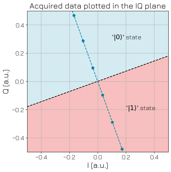
We proceed next to the thresholded acquisition. Since we want to separate positive and negative real parts, we set the threshold to 0. With the previous fit of the raw data, we also already computed the value angle_cutoff from which the data should be rotated before comparison.
[32]:
from qblox_scheduler import ClockResource, Schedule
from qblox_scheduler.operations import SquarePulse, ThresholdedAcquisition
from qblox_scheduler.operations.loop_domains import DType, linspace

THRESHOLD: float = 0.0

thres_acq_sched: Schedule = Schedule("thresholded_acquisition")
thres_acq_sched.add_resource(ClockResource(name="clock", freq=80e6))

with thres_acq_sched.loop(linspace(-1.0, 1.0, 6, dtype=DType.AMPLITUDE)) as amp:
    thres_acq_sched.add(
        SquarePulse(
            duration=PULSE_DURATION,
            amplitude=amp,
            port="q0:port",
            clock="clock",
        ),
    )
    thres_acq_sched.add(
        ThresholdedAcquisition(
            duration=ACQ_DURATION,
            port="q0:port",
            clock="clock",
            acq_channel="data",
            acq_rotation=angle_cutoff,
            acq_threshold=THRESHOLD,
            coords={"amp": amp},
        ),
        ref_pt="start",
        rel_time=TIME_OF_FLIGHT,
    )

xr_data_thresholded: xarray.Dataset = hardware_agent.run(thres_acq_sched)
[33]:
import xarray as xr

xr_data_thresholded = xr.open_dataset("./utils/data/data_thresholded.hdf5", engine="h5netcdf")
# lazy loading
xr_data_thresholded.coords["amp"].values
xr_data_thresholded.data.data
[33]:
array([0., 0., 0., 1., 1., 1.])
[34]:
xr_data_thresholded
[34]:
<xarray.Dataset> Size: 192B
Dimensions:               (acq_index_data: 6)
Coordinates:
  * acq_index_data        (acq_index_data) int64 48B 0 1 2 3 4 5
    loop_repetition_data  (acq_index_data) float64 48B ...
    amp                   (acq_index_data) float64 48B -1.0 -0.6 ... 0.6 1.0
Data variables:
    data                  (acq_index_data) float64 48B 0.0 0.0 0.0 1.0 1.0 1.0
Attributes:
tuid: 20250926-113721-667-940776As expected, the 3 first points are identified as being in the 0 state (I values below threshold), and the 3 last points are indeed in the 1 state (above threshold).
Trigger count acquisition#
The trigger count acquisition protocol is used for measuring how many times the input signal goes over some limit. This protocol is used, for example, in cases where one wants to count the number of detection events in an experiment.
The trigger count protocol is currently only available on two module types: the QRM (baseband) and the QTM.
Similarly to what was discussed above with the single-sideband integration acquisition protocol, we can make use of the coords argument to append and/or sum the number of trigger events received during a given acquisition window. If a loop reference is set as being a coordinate of the acquisition, the number of counts is appended is appended at each iteration of the loop.
In addition to the integration and appending bin modes the TriggerCount protocol offers the distribution bin mode, which can only be used with the QRM.
In the distribution bin mode, the result is a distribution that maps the trigger count numbers to the number of occurrences of each trigger count number. This provides insights into the overall occurrence of triggers when running the acquisition multiple times. For example, imagine an experiment where a TriggerCount acquisition runs three times and detects [1, 3, 1] triggers respectively. In distribution mode, the instrument directly compiles a histogram of these results. It would
report that a count of ‘1’ occurred twice and a count of ‘3’ occurred once, returning a result like {1: 2, 3: 1}. The dictionary notation shows the number of triggers as keys and their corresponding frequencies as values.
{note} The threshold is set for the QRM via the [TTL acquisition threshold field](../../user_guide/hardware_config.md#sequencer-options), while for the QTM this threshold is set via the field `analog_threshold` in the [digitization threshold hardware option](../../user_guide/hardware_config.md#digitization-thresholds).
Setup and schedule#
Let’s have an illustrative example showing how this type of acquisition works in practice.
We use a source of random dirac pulses that we made up with a function generator: it plays a 20ns wide TTL pulse in burst mode, externally triggered with a source of noise. The ratio between the burst trigger level of the function generator, and the RMS amplitude of the noise sets the average flux of pulses emitted by the source. In practice we set it up to have a flux of a few pulses per micro-second.
This source of random pulses is then connected to the second input of a QRM module, to proceed to the detection and counting.
Let’s first set up the hardware configuration for this experiment. We will set up the counting threshold of the QRM to 60% of the maximum input amplitude (so 0.6 x 0.5V = 300mV).
We will perform the acquisitions in a window of 15us:
[35]:
ACQ_DURATION: float = 15e-6
[36]:
hardware_cfg_trigger_count: dict[str, Any] = {
    "config_type": "QbloxHardwareCompilationConfig",
    "version": "0.2",
    "hardware_description": {
        "cluster0": {
            "instrument_type": "Cluster",
            "modules": {
                4: {"instrument_type": "QRM"},
            },
            "ref": "internal",
        },
    },
    "hardware_options": {
        "sequencer_options": {
            "qrm:in1-digital": {
                "ttl_acq_threshold": 0.6,
            }
        },
    },
    "connectivity": {
        "graph": [
            ["cluster0.module4.complex_output_0", "qrm:out"],
            ["cluster0.module4.real_input_0", "qrm:in0"],
            ["cluster0.module4.real_input_1", "qrm:in1"],
        ]
    },
}

hardware_agent: HardwareAgent = HardwareAgent(hardware_configuration=hardware_cfg_trigger_count)
hardware_agent.connect_clusters()
/.venv/lib/python3.14/site-packages/qblox_scheduler/qblox/hardware_agent.py:556: UserWarning: cluster0: Trying to instantiate cluster with ip 'None'.Creating a dummy cluster.
  warnings.warn(
/.venv/lib/python3.14/site-packages/qblox_instruments/ieee488_2/cluster_dummy_transport.py:590: RuntimeWarning: coroutine 'DummyTransport.close' was never awaited
  mod.close()
RuntimeWarning: Enable tracemalloc to get the object allocation traceback
First check: scope acquisition#
We will start by simply performing a scope acquisition of the signal, to verify how it looks.
[37]:
from qblox_scheduler import Schedule
from qblox_scheduler.operations import Trace

schedule: Schedule = Schedule("trace_acquisition_tutorial")

schedule.add(
    Trace(duration=ACQ_DURATION, acq_channel="scope", port="qrm:in1", clock="cl0.baseband")
)

xr_ttl_trace_acquisition: xarray.Dataset = hardware_agent.run(schedule)
Invalid input indices are connected. Scope data might be invalid. Connected input indices are (1,). Valid indices are (0, 1) and (2, 3).
[38]:
import xarray as xr

xr_ttl_trace_acquisition = xr.open_dataset(
    "./utils/data/trigger_count_scope.hdf5", engine="h5netcdf"
)
[39]:
import matplotlib.pyplot as plt

fig, ax = plt.subplots(figsize=(10, 4))

xr_ttl_trace_acquisition["scope"].imag.plot(ax=ax)

ax.set_xlabel("Time (ns)")
ax.set_ylabel("Amplitude (a.u.)")
ax.set_title("Acquired trace")
ax.set_ylim(-0.1, 1.0)
ax.grid()
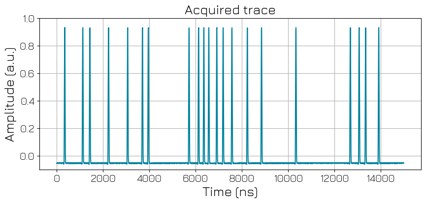
Appending the counts#
We will repeat a TriggerCount acquisition, appending all the result until we entirely filled the instrument memory (currently set to a maximum of 131_072 bins).
[40]:
from qblox_scheduler import Schedule
from qblox_scheduler.operations import TriggerCount
from qblox_scheduler.operations.loop_domains import DType

REPS: int = 131_072  # maximum number of bins usable on instrument memory

schedule: Schedule = Schedule("trigger_count_acquisition_tutorial")

with schedule.loop(arange(0, REPS, 1, dtype=DType.NUMBER)) as rep:
    schedule.add(
        TriggerCount(
            duration=ACQ_DURATION,
            port="qrm:in1",
            clock="cl0.baseband",
            acq_channel="counts",
            coords={"rep": rep},
        )
    )
xr_ttl_append_counts_acquisition: xarray.Dataset = hardware_agent.run(schedule)
[41]:
import xarray as xr

xr_ttl_append_counts_acquisition = xr.open_dataset(
    "./utils/data/trigger_count_append.hdf5", engine="h5netcdf"
)
Let’s now plot the histogram of the 131k appended counts, as well as the gaussian that we can extract from the computation of the mean value and standard deviation of this data series.
[42]:
fig, ax = plt.subplots()

avg = xr_ttl_append_counts_acquisition["counts"].mean().item()
std = xr_ttl_append_counts_acquisition["counts"].std().item()

x = np.linspace(0, 40, 100)
y = np.exp(-0.5 * ((x - avg) / std) ** 2) * REPS / (std * np.sqrt(2 * np.pi))

xr_ttl_append_counts_acquisition["counts"].plot.hist(
    bins=list(range(41)), edgecolor="black", align="left", ax=ax, label="Appended data histogram"
)
ax.plot(x, y, color="tab:red", ls="dashed", lw=2, label="Gaussian fit")


ax.legend()
ax.set_xlabel("Counts")
ax.set_ylabel("Occurrences")
ax.set_title(f"Histogram of Trigger Counts over {REPS} repetitions")
ax.text(30, 6000, f"Mean: {avg:.2f}\nStd: {std:.2f}")
[42]:
Text(30, 6000, 'Mean: 19.43\nStd: 3.72')
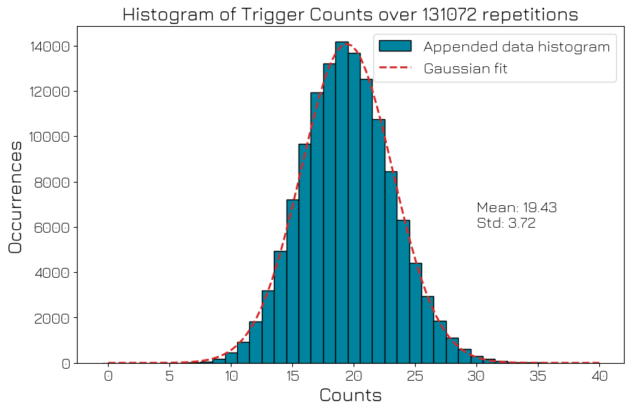
We therefore measured a flux of \(1.3 \pm 0.2\) pulse/sec
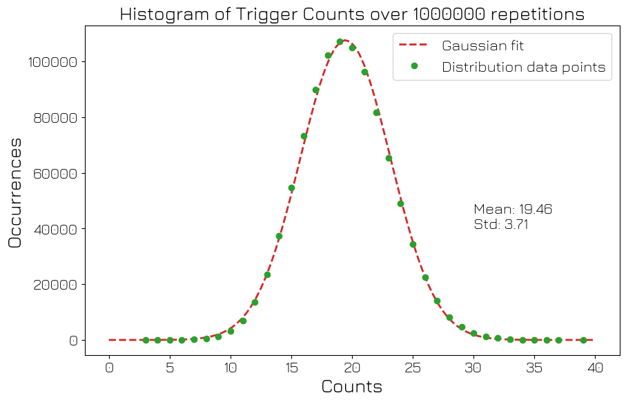
Distribution mode#
From what was explained before, it is clear that above histogram could have been obtained in one step (i.e. without data analysis function) using the distribution bin mode.
Not only it spares us from doing any post-analysis of the raw data (the histogram binning is happening on the instrument side), but also – and more importantly – we no longer saturates the instrument memory, meaning that the acquisition can be iterated much longer: let’s do it for a million of iteration.
[43]:
from qblox_scheduler import Schedule
from qblox_scheduler.operations import TriggerCount
from qblox_scheduler.operations.acquisition_library import BinMode
from qblox_scheduler.operations.loop_domains import DType

REPS: int = 1_000_000  # maximum number of bins usable on instrument memory

schedule: Schedule = Schedule("trigger_count_acquisition_tutorial")

with schedule.loop(arange(0, REPS, 1, dtype=DType.NUMBER)) as rep:
    schedule.add(
        TriggerCount(
            duration=ACQ_DURATION,
            port="qrm:in1",
            clock="cl0.baseband",
            acq_channel="occurrence",
            bin_mode=BinMode.DISTRIBUTION,
        )
    )
xr_data_distr: xarray.Dataset = hardware_agent.run(schedule)
[44]:
import xarray as xr

xr_data_distr = xr.open_dataset("./utils/data/trigger_count_distr.hdf5", engine="h5netcdf")
[45]:
fig, ax = plt.subplots()

avg = np.average(xr_data_distr["counts_occurrence"], weights=xr_data_distr["occurrence"]).item()
std = np.sqrt(
    np.average((xr_data_distr["counts_occurrence"] - avg) ** 2, weights=xr_data_distr["occurrence"])
).item()

x = np.linspace(0, 40, 100)
y = np.exp(-0.5 * ((x - avg) / std) ** 2) * REPS / (std * np.sqrt(2 * np.pi))

ax.plot(x, y, color="tab:red", ls="dashed", lw=2, label="Gaussian fit")
xr_data_distr["occurrence"].plot(
    x="counts_occurrence",
    marker="o",
    ls="None",
    color="tab:green",
    ax=ax,
    label="Distribution data points",
)


ax.legend()
ax.set_xlabel("Counts")
ax.set_ylabel("Occurrences")
ax.set_title(f"Histogram of Trigger Counts over {REPS} repetitions")
ax.text(30, 40000, f"Mean: {avg:.2f}\nStd: {std:.2f}")
[45]:
Text(30, 40000, 'Mean: 19.46\nStd: 3.71')
[46]:
avg = 19.43
std = 3.71


def gaussian(x):
    return np.exp(-0.5 * ((x - avg) / std) ** 2) / (std * np.sqrt(2 * np.pi))


x = np.linspace(0, 40, 1000)
y = gaussian(x)

fig, ax = plt.subplots(figsize=(10, 5))
# vertical line at 17 below the curve
ax.axvline(17, color="red", ls="dashed", lw=2, ymin=0.04, ymax=0.78, label="Movable threshold")
ax.plot(x, y, color="k", lw=2)


# shade area under the curve to the left of 17
x_fill_left = np.linspace(0, 17, 200)
y_fill_left = y = gaussian(x_fill_left)

x_fill_right = np.linspace(17, 40, 200)
y_fill_right = y = gaussian(x_fill_right)

ax.fill_between(
    x_fill_left,
    y_fill_left,
    color="lightgreen",
    alpha=0.5,
    label="Below threshold $\\rightarrow$ 1",
)
ax.fill_between(
    x_fill_right,
    y_fill_right,
    color="lightblue",
    alpha=0.5,
    label="Above threshold $\\rightarrow$ 0",
)

ax.set_xlabel("Counts")
ax.set_ylabel("Probability density")
ax.grid()
ax.legend()

plt.savefig("./utils/images/thresholded_acquisition_schematic.png", dpi=300)
plt.close(fig)
Thresholded trigger count acquisition#
Generalities#
The thresholded trigger count protocol combines the functionality of the trigger count acquisition with a final comparison step. It first counts the rising edges of an input signal over a duration and then compares this total count to a specified integer threshold. The threshold comparison result (False (0), or True (1)) can be retrieved directly, and can also be used to conditionally execute other instructions. For the latter, you would use the ConditionalOperation.
We propose here to keep using our source of random pulses for illustrating this acquisition protocol. We still use 15us long acquisition windows, within which the pulses are counted. As shown in the figure below, if the number of counts is smaller than the threshold, we trigger an event on the cluster internal network, and we count the acquisition as a 1, otherwise no event is triggered and we count it as a 0.
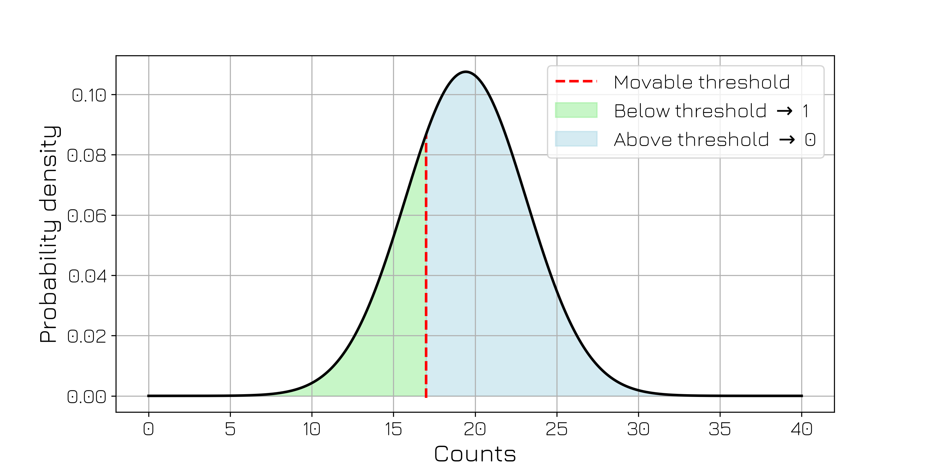
By scanning over the value \(n_{th}\) of the threshold, the probability \(P_1(n_{th})\) of having the acquisition returning 1 should follow the erf error function, corresponding the antiderivative of the gaussian.
Schedule and verification with an oscilloscope#
The source of pulses is connected to the input 1 of the QRM. An oscilloscope is connected to the output channels of the QRM, for checking if the conditionally triggered operation are correctly executed. We start by writing a simple schedule:
a 1us long square pulse is played by the QRM: it is used to trigger a single acquisition with the oscilloscope;
we wait 1us;
the acquisition starts, it lasts 15us and an event is send on the trigger network (label “click”) if at least 1 count has been detected: regarding the typical number of pulses detected in 15us (see above), this effectively ensures the emission of an event;
a negative square pulse is played, triggered by the event on the “click” channel;
[47]:
from qblox_scheduler import Schedule
from qblox_scheduler.operations import (
    ConditionalOperation,
    IdlePulse,
    SquarePulse,
    ThresholdedTriggerCount,
)

schedule: Schedule = Schedule("Conditional operation")
schedule.add(SquarePulse(amplitude=1, duration=1e-6, port="qrm:out", clock="cl0.baseband"))
schedule.add(IdlePulse(duration=1e-6))
schedule.add(
    ThresholdedTriggerCount(
        port="qrm:in1",
        clock="cl0.baseband",
        duration=15e-6,
        threshold=1,  # very small threshold to ensure a trigger
        feedback_trigger_label="click",  # label of the trigger to be used in the ConditionalOperation
    )
)
schedule.add(
    ConditionalOperation(
        body=SquarePulse(amplitude=-1, duration=1e-6, port="qrm:out", clock="cl0.baseband"),
        qubit_name="click",
    ),
)
schedule.add(IdlePulse(4e-9))
[47]:
{'name': '1cbd81bf-2792-4571-a015-91f9e592444c', 'operation_id': '5283007011841464040', 'timing_constraints': [TimingConstraint(ref_schedulable=None, ref_pt=None, ref_pt_new=None, rel_time=0)], 'label': '1cbd81bf-2792-4571-a015-91f9e592444c'}
[48]:
import numpy as np
from matplotlib import pyplot as plt

scope_data = np.genfromtxt(
    "./utils/data/conditional_playback_wf.csv",
    delimiter=",",
    skip_header=12,
)


fig, ax = plt.subplots(figsize=(12, 4))

arr_time, arr_trace = scope_data[:, 0], scope_data[:, 1]

ax.axvspan(1, 2, color="pink", alpha=0.5)
ax.axvspan(2, 17, color="tab:green", alpha=0.2)
ax.text(9.5, 0.25, "Acquisition", fontsize=12, ha="center", color="green")
ax.plot(arr_time * 1e6, arr_trace)

ax.set_xlabel("Time (us)")
ax.set_ylabel("Amplitude (V)")
ax.set_title("Acquired trace after conditional operation triggered")
ax.grid()

plt.tight_layout()
plt.savefig("./utils/images/conditional_playback_trace.png", dpi=300)
plt.close(fig)
Let’s plot the trace acquired by the scope is indeed showing two pulses of opposite polarities, and check that the duration between both pulses is indeed the expected one:
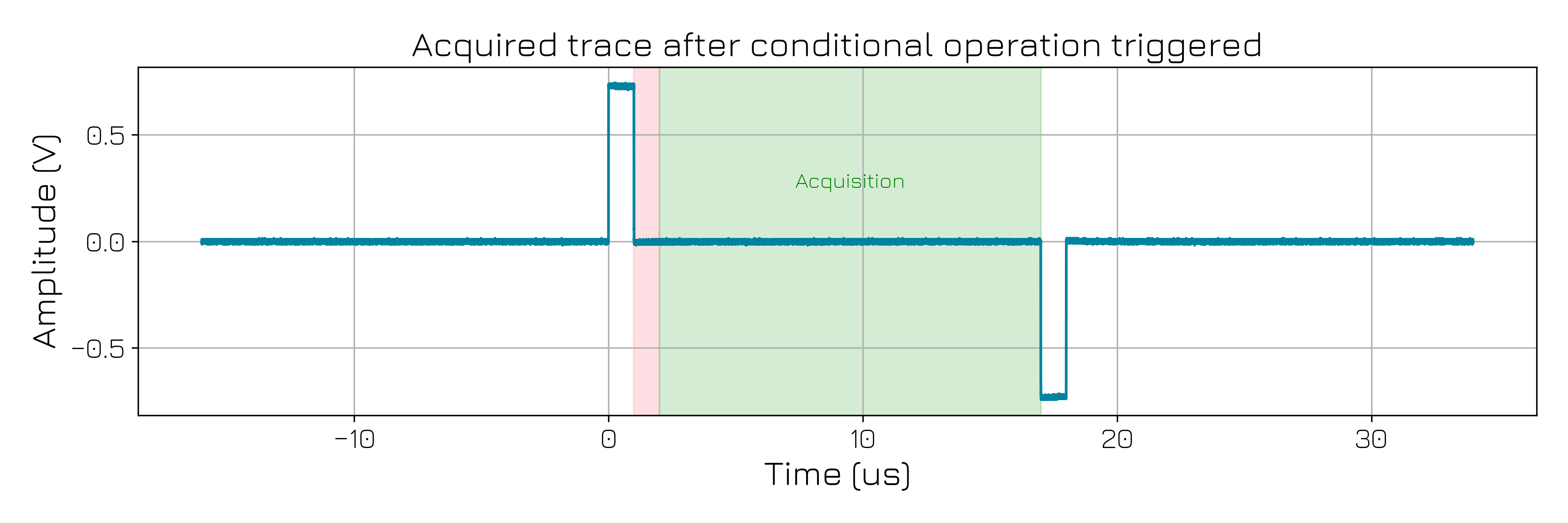
[49]:
threshold: float = 0.5
above_threshold: np.ndarray = arr_trace > threshold
below_threshold: np.ndarray = arr_trace < -threshold
first_pulse_timestamp: int = np.where(above_threshold)[0][0]
second_pulse_timestamp: int = np.where(below_threshold)[0][0]
delta_t: int = arr_time[second_pulse_timestamp] - arr_time[first_pulse_timestamp]
print(f"Delay time between pulses: {delta_t * 1e6:.1f} us")
Delay time between pulses: 17.0 us
Let’s now proceed to the complete experiment, where the threshold value is scanned, and for each value of the threshold we perform 100_000 iteration of the ThresholdedTriggerCount acquisition.
[50]:
from qblox_scheduler import Schedule
from qblox_scheduler.enums import TriggerCondition
from qblox_scheduler.operations import (
    ConditionalOperation,
    IdlePulse,
    SquarePulse,
    ThresholdedTriggerCount,
)

datasets: list[xarray.Dataset] = []
for threshold in range(40):
    schedule: Schedule = Schedule("Conditional operation")

    schedule.add(SquarePulse(amplitude=1, duration=1e-6, port="qrm:out", clock="cl0.baseband"))
    schedule.add(IdlePulse(duration=1e-6))

    with schedule.loop(arange(0, 100_000, 1, dtype=DType.NUMBER)) as rep:
        schedule.add(
            ThresholdedTriggerCount(
                port="qrm:in1",
                clock="cl0.baseband",
                duration=15e-6,
                threshold=threshold,
                feedback_trigger_label="click",
                acq_channel="thresholded_count",
                feedback_trigger_condition=TriggerCondition.LESS_THAN,
            )
        )
        schedule.add(
            ConditionalOperation(
                body=SquarePulse(amplitude=-1, duration=1e-6, port="qrm:out", clock="cl0.baseband"),
                qubit_name="click",
            ),
        )
        schedule.add(IdlePulse(4e-9))

    datasets.append(hardware_agent.run(schedule))
[51]:
import pickle as pkl
from pathlib import Path

source_file = Path("./utils/data/datasets.pkl")
with source_file.open("rb") as f:
    datasets = pkl.load(f)
[52]:
cumulative_probability: list[float] = []
for dataset in datasets:
    cumulative_probability.append(dataset.thresholded_count.sum().item() / 100_000)

fig, ax = plt.subplots(figsize=(10, 5))
ax.plot(range(40), cumulative_probability, marker="o")
ax.set_xlabel("Threshold")
ax.set_ylabel("Probability")
ax.set_title("Cumulative probability to detect a trigger vs threshold")
ax.grid()