See also

A Jupyter notebook version of this tutorial can be downloaded here.

Operations and qubits

Gates, measurements and qubits

In the previous tutorials, experiments were created on the quantum-device level. On this level, operations are defined in terms of explicit signals and locations on the chip, rather than the qubit and the intended operation. To work at a greater level of abstraction, qblox-scheduler allows creating operations on the quantum-circuit level. Instead of signals, clocks, and ports, operations are defined by the effect they have on specific qubits. This representation of the schedules can be compiled to the quantum-device level to create the pulse schemes.

In this tutorial we show how to define operations on the quantum-circuit level, combine them into schedules, and show their circuit-level visualization. We go through the configuration file needed to compile the schedule to the quantum-device level and show how these configuration files can be created automatically and dynamically.

Many of the gates used in the circuit layer description are defined in qblox_scheduler.operations.gate_library such as qblox_scheduler.operations.gate_library.Reset, qblox_scheduler.operations.gate_library.X90 and qblox_scheduler.operations.gate_library.Measure. Operations are instantiated by providing them with the name of the qubit(s) on which they operate:

from qblox_scheduler.operations import CZ, X90, Measure, Reset

q0, q1 = ("q0", "q1")
X90(q0)
Measure(q1)
CZ(q0, q1)
Reset(q0)

{'name': 'Reset q0', 'gate_info': {'unitary': None, 'tex': '$|0\\rangle$', 'plot_func': 'qblox_scheduler.schedules._visualization.circuit_diagram.reset', 'device_elements': ['q0'], 'operation_type': 'reset', 'device_overrides': {}}, 'pulse_info': [], 'acquisition_info': [], 'logic_info': {}, 'statement_info': {}}

Within a single qblox_scheduler.schedules.schedule.Schedule, high-level circuit layer operations can be mixed with quantum-device level operations. This mixed representation is useful for experiments where some pulses cannot easily be represented as qubit gates. An example of this is given by the Chevron experiment given in Mixing pulse and circuit layer operations.

Circuit layer schedule example: Bell test

We demonstrate the extra layer of abstraction that circuit-level operations offer by creating a qblox_scheduler.schedules.schedule.Schedule for measuring Bell violations.

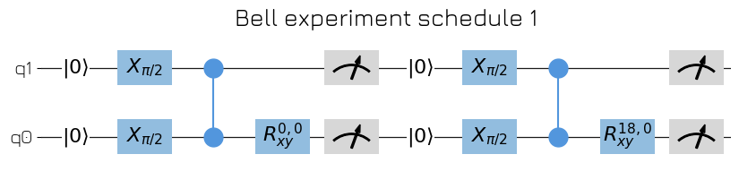
As the first example, we want to create a schedule for performing the Bell experiment. The goal of the Bell experiment is to create a Bell state \(|\Phi ^+\rangle=\frac{1}{2}(|00\rangle+|11\rangle)\) which is a perfectly entangled state, followed by a measurement. By rotating the measurement basis, or equivalently one of the qubits, it is possible to observe violations of the CSHS inequality.

We create this experiment using the quantum-circuit level description. This allows defining the Bell schedule as:

import numpy as np

from qblox_scheduler import Schedule
from qblox_scheduler.operations import CZ, X90, Measure, Reset, Rxy

sched = Schedule("Bell experiment")

for acq_idx, theta in enumerate(np.linspace(0, 360, 21)):
    sched.add(Reset(q0, q1))
    sched.add(X90(q0))
    sched.add(X90(q1), ref_pt="start")  # Start at the same time as the other X90
    sched.add(CZ(q0, q1))
    sched.add(Rxy(theta=theta, phi=0, qubit=q0))

    sched.add(Measure(q0, acq_index=acq_idx), label=f"M q0 {theta:.2f} deg")
    sched.add(
        Measure(q1, acq_index=acq_idx),
        label=f"M q1 {theta:.2f} deg",
        ref_pt="start",  # Start at the same time as the other measure
    )

sched

<qblox_scheduler.schedule.Schedule at 0x7fb2faaaf820>

Visualizing the quantum circuit

We can directly visualize the created schedule on the quantum-circuit level with the qblox_scheduler.schedules.schedule.ScheduleBase.plot_circuit_diagram method. This visualization shows every operation on a line representing the different qubits.

import matplotlib.pyplot as plt

_, ax = sched.plot_circuit_diagram()
# all gates are plotted, but it doesn't all fit in a matplotlib figure.
# Therefore we use :code:`set_xlim` to limit the number of gates shown.
ax.set_xlim(-0.5, 9.5)
plt.show()

In previous tutorials, we visualized the schedules on the pulse level using qblox_scheduler.schedules.schedule.ScheduleBase.plot_pulse_diagram . Up until now, however, all gates have been defined on the quantum-circuit level without defining the corresponding pulse shapes. Therefore, trying to run qblox_scheduler.schedules.schedule.ScheduleBase.plot_pulse_diagram will raise an error which signifies no pulse_info is present in the schedule:

sched.plot_pulse_diagram()

---------------------------------------------------------------------------
KeyError                                  Traceback (most recent call last)
Cell In[4], line 1
----> 1 sched.plot_pulse_diagram()

File /builds/1/.venv/lib/python3.10/site-packages/qblox_scheduler/schedule.py:450, in Schedule.plot_pulse_diagram(self, port_list, sampling_rate, modulation, modulation_if, plot_backend, x_range, combine_waveforms_on_same_port, timeable_schedule_index, **backend_kwargs)
    448         raise IndexError(f"No timeable schedule at index {timeable_schedule_index}")
    449     timeable_schedule = timeable_schedules[timeable_schedule_index]
--> 450 return timeable_schedule.plot_pulse_diagram(
    451     port_list,
    452     sampling_rate,
    453     modulation,
    454     modulation_if,
    455     plot_backend,
    456     x_range,
    457     combine_waveforms_on_same_port,
    458     **backend_kwargs,
    459 )

File /builds/1/.venv/lib/python3.10/site-packages/qblox_scheduler/schedules/schedule.py:439, in TimeableScheduleBase.plot_pulse_diagram(self, port_list, sampling_rate, modulation, modulation_if, plot_backend, x_range, combine_waveforms_on_same_port, **backend_kwargs)
    435 # NB imported here to avoid circular import
    437 from qblox_scheduler.schedules._visualization.pulse_diagram import sample_schedule
--> 439 sampled_pulses_and_acqs = sample_schedule(
    440     self,
    441     sampling_rate=sampling_rate,
    442     port_list=port_list,
    443     modulation=modulation,
    444     modulation_if=modulation_if,
    445     x_range=x_range,
    446     combine_waveforms_on_same_port=combine_waveforms_on_same_port,
    447 )
    449 if plot_backend == "mpl":
    450     # NB imported here to avoid circular import
    452     from qblox_scheduler.schedules._visualization.pulse_diagram import (
    453         pulse_diagram_matplotlib,
    454     )

File /builds/1/.venv/lib/python3.10/site-packages/qblox_scheduler/schedules/_visualization/pulse_diagram.py:457, in sample_schedule(schedule, port_list, modulation, modulation_if, sampling_rate, x_range, combine_waveforms_on_same_port)
    454 pulse_infos: dict[str, list[ScheduledInfo]] = defaultdict(list)
    455 acq_infos: dict[str, list[ScheduledInfo]] = defaultdict(list)
--> 457 _extract_schedule_infos(
    458     schedule,
    459     port_list,
    460     0,
    461     offset_infos,
    462     pulse_infos,
    463     acq_infos,
    464 )
    466 x_min, x_max = x_range
    468 sampled_pulses = get_sampled_pulses_from_voltage_offsets(
    469     schedule=schedule,
    470     offset_infos=offset_infos,
   (...)
    474     modulation_if=modulation_if,
    475 )

File /builds/1/.venv/lib/python3.10/site-packages/qblox_scheduler/schedules/_visualization/pulse_diagram.py:355, in _extract_schedule_infos(operation, port_list, time_offset, offset_infos, pulse_infos, acq_infos)
    353     for schedulable in operation.schedulables.values():
    354         inner_operation = operation.operations[schedulable["operation_id"]]
--> 355         abs_time = schedulable["abs_time"]
    356         _extract_schedule_infos(
    357             inner_operation,
    358             port_list,
   (...)
    362             acq_infos,
    363         )
    364 elif isinstance(operation, ConditionalOperation):

File /usr/local/lib/python3.10/collections/__init__.py:1106, in UserDict.__getitem__(self, key)
   1104 if hasattr(self.__class__, "__missing__"):
   1105     return self.__class__.__missing__(self, key)
-> 1106 raise KeyError(key)

KeyError: 'abs_time'

And similarly for the timing_table:

sched.timing_table

---------------------------------------------------------------------------
ValueError                                Traceback (most recent call last)
Cell In[5], line 1
----> 1 sched.timing_table

File /builds/1/.venv/lib/python3.10/site-packages/qblox_scheduler/schedule.py:554, in Schedule.timing_table(self)
    552 if timeable_schedule is None:
    553     raise ValueError("can not plot timing table for schedules with untimed operations")
--> 554 return timeable_schedule.timing_table

File /builds/1/.venv/lib/python3.10/site-packages/qblox_scheduler/schedules/schedule.py:628, in TimeableScheduleBase.timing_table(self)
    534 """
    535 A styled pandas dataframe containing the absolute timing of pulses and acquisitions in a schedule.
    536
   (...)
    625
    626 """  # noqa: E501
    627 timing_table_list = []
--> 628 self._generate_timing_table_list(self, 0, timing_table_list, None)
    629 timing_table = pd.concat(timing_table_list, ignore_index=True)
    630 timing_table = timing_table.sort_values(by="abs_time")

File /builds/1/.venv/lib/python3.10/site-packages/qblox_scheduler/schedules/schedule.py:489, in TimeableScheduleBase._generate_timing_table_list(cls, operation, time_offset, timing_table_list, operation_id)
    486     for schedulable in operation.schedulables.values():
    487         if "abs_time" not in schedulable:
    488             # when this exception is encountered
--> 489             raise ValueError(
    490                 "Absolute time has not been determined yet. Please compile your schedule."
    491             )
    492         cls._generate_timing_table_list(
    493             operation.operations[schedulable["operation_id"]],
    494             time_offset + schedulable["abs_time"],
    495             timing_table_list,
    496             schedulable["operation_id"],
    497         )
    498 elif isinstance(operation, LoopOperation):

ValueError: Absolute time has not been determined yet. Please compile your schedule.

Quantum devices and elements

The device configuration contains all knowledge of the physical device under test (DUT). To generate these device configurations on the fly, qblox-scheduler provides the qblox_scheduler.device_under_test.quantum_device.QuantumDevice and qblox_scheduler.device_under_test.device_element.DeviceElement classes.

These classes contain the information necessary to generate the device configs and allow changing their parameters on-the-fly. The qblox_scheduler.device_under_test.quantum_device.QuantumDevice class represents the DUT containing different qblox_scheduler.device_under_test.device_element.DeviceElement s. Currently, qblox-scheduler contains the qblox_scheduler.device_under_test.transmon_element.BasicTransmonElement class to represent a fixed-frequency transmon qubit connected to a feedline. We show their interaction below:

from qblox_scheduler import BasicTransmonElement, QuantumDevice

# First create a device under test
dut = QuantumDevice("DUT")

# Then create a transmon element
qubit = BasicTransmonElement("qubit")

# Finally, add the transmon element to the QuantumDevice
dut.add_element(qubit)
dut, dut.elements

(QuantumDevice(name='DUT', elements={'qubit': BasicTransmonElement(name='qubit', element_type='BasicTransmonElement', reset=IdlingReset(name='reset', duration=0.0002), rxy=RxyDRAG(name='rxy', amp180=nan, beta=0.0, duration=2e-08, reference_magnitude=ReferenceMagnitude(name='reference_magnitude', dBm=nan, V=nan, A=nan)), measure=DispersiveMeasurement(name='measure', pulse_type='SquarePulse', pulse_amp=0.25, pulse_duration=3e-07, acq_channel=0, acq_delay=0.0, integration_time=1e-06, reset_clock_phase=True, acq_weights_a=array([], dtype=float64), acq_weights_b=array([], dtype=float64), acq_weights_sampling_rate=1000000000.0, acq_weight_type='SSB', acq_rotation=0.0, acq_threshold=0.0, num_points=1, reference_magnitude=ReferenceMagnitude(name='reference_magnitude', dBm=nan, V=nan, A=nan)), pulse_compensation=PulseCompensationModule(name='pulse_compensation', max_compensation_amp=nan, time_grid=nan, sampling_rate=nan), ports=Ports(name='ports', microwave='qubit:mw', flux='qubit:fl', readout='qubit:res'), clock_freqs=ClocksFrequencies(name='clock_freqs', f01=nan, f12=nan, readout=nan))}, edges={}, instr_instrument_coordinator=None, cfg_sched_repetitions=1024, keep_original_schedule=True, hardware_config=None, scheduling_strategy=<SchedulingStrategy.ASAP: 'asap'>),
 {'qubit': BasicTransmonElement(name='qubit', element_type='BasicTransmonElement', reset=IdlingReset(name='reset', duration=0.0002), rxy=RxyDRAG(name='rxy', amp180=nan, beta=0.0, duration=2e-08, reference_magnitude=ReferenceMagnitude(name='reference_magnitude', dBm=nan, V=nan, A=nan)), measure=DispersiveMeasurement(name='measure', pulse_type='SquarePulse', pulse_amp=0.25, pulse_duration=3e-07, acq_channel=0, acq_delay=0.0, integration_time=1e-06, reset_clock_phase=True, acq_weights_a=array([], dtype=float64), acq_weights_b=array([], dtype=float64), acq_weights_sampling_rate=1000000000.0, acq_weight_type='SSB', acq_rotation=0.0, acq_threshold=0.0, num_points=1, reference_magnitude=ReferenceMagnitude(name='reference_magnitude', dBm=nan, V=nan, A=nan)), pulse_compensation=PulseCompensationModule(name='pulse_compensation', max_compensation_amp=nan, time_grid=nan, sampling_rate=nan), ports=Ports(name='ports', microwave='qubit:mw', flux='qubit:fl', readout='qubit:res'), clock_freqs=ClocksFrequencies(name='clock_freqs', f01=nan, f12=nan, readout=nan))})

The different transmon properties can be set through attributes of the qblox_scheduler.device_under_test.transmon_element.BasicTransmonElement class instance, e.g.:

qubit.clock_freqs.f01 = 6e9

Mixing pulse and circuit layer operations

We can mix the circuit layer representation with pulse-level operations, which can be useful for experiments involving pulses not easily represented by gates.

from qblox_scheduler import ClockResource, Schedule
from qblox_scheduler.operations import X90, Measure, Reset, SquarePulse, X

sched = Schedule("Experiment with both pulse and circuit layer operations")

reset = sched.add(Reset("q0"))
sched.add(X("q0"), ref_op=reset, ref_pt="end")  # Start at the end of the reset
# We specify a clock for tutorial purposes
square = sched.add(SquarePulse(amp=0.1, duration=1e-6, port="q0:mw", clock="q0.01"))
sched.add(Measure(q0, coords={"amplitude": 0.1}, acq_channel="S_21"), label="M q0")

# Specify the frequencies for the clocks; this can also be done via the DeviceElement (BasicTransmonElement) instead
sched.add_resources(
    [
        ClockResource("q0.01", 6.02e9),
        ClockResource("q0.ro", 5.02e9),
    ]
)

sched.plot_circuit_diagram()

(<Figure size 1000x100 with 1 Axes>,
 <Axes: title={'center': 'Experiment with both pulse and circuit layer operations schedule 1'}>)

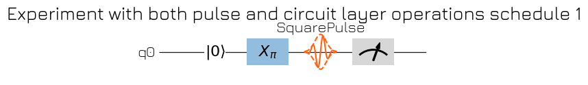
This example shows that we add gates using the same interface as pulses. Gates are Operations, and as such support the same timing and reference operators as Pulses.

Schedule compilation with the HardwareAgent

The HardwareAgent is responsible for instantiating everything that is necessary to run an experiment, as well as actually running the experiment. A hardware configuration is required, but a device configuration is not. The Compiling to Hardware section demonstrates how to set the hardware configuration.

from qblox_scheduler import BasicTransmonElement, HardwareAgent, QuantumDevice

dut.close()
dut = QuantumDevice("DUT")
q0_dev = BasicTransmonElement("q0")
q1_dev = BasicTransmonElement("q1")
dut.add_element(q0_dev)
dut.add_element(q1_dev)
dut.get_element("q0").clock_freqs.f01 = 4e9
dut.get_element("q0").rxy.amp180 = 0.65
dut.get_element("q1").rxy.amp180 = 0.55
dut.get_element("q0").measure.pulse_amp = 0.28
dut.get_element("q1").measure.pulse_amp = 0.22

agent = HardwareAgent("./dependencies/configs/hw_cfg.json", dut)

compiled_sched = agent.compile(schedule=sched)

/tmp/ipykernel_18185/408239406.py:3: UserWarning: QuantumDevice is not an instrument, no need to close it!
  dut.close()
/builds/1/.venv/lib/python3.10/site-packages/qblox_scheduler/backends/circuit_to_device.py:439: RuntimeWarning: Clock 'q0.01' has conflicting frequency definitions: 6020000000.0 Hz in the schedule and 4000000000.0 Hz in the device config. The clock is set to '6020000000.0'. Ensure the schedule clock resource matches the device config clock frequency or set the clock frequency in the device config to np.NaN to omit this warning.
  warnings.warn(

So, finally, we can show the timing table associated with the Chevron schedule and plot its pulse diagram:

compiled_sched.timing_table.hide(slice(11, None), axis="index").hide(
    "waveform_op_id", axis="columns"
)

	port	clock	abs_time	duration	is_acquisition	operation	wf_idx	operation_hash
0	None	cl0.baseband	0.0 ns	200,000.0 ns	False	Reset('q0')	0	1522317815387438915
1	q0:mw	q0.01	200,000.0 ns	20.0 ns	False	X(qubit='q0')	0	-3006420249231672064
2	q0:mw	q0.01	200,020.0 ns	1,000.0 ns	False	SquarePulse(amp=0.1,duration=1e-06,port='q0:mw',clock='q0.01',reference_magnitude=None,t0=0)	0	6003854298736714017
3	None	q0.ro	201,020.0 ns	0.0 ns	False	ResetClockPhase(clock='q0.ro',t0=0)	0	4185216258086596527
4	q0:res	q0.ro	201,020.0 ns	300.0 ns	False	SquarePulse(amp=0.28,duration=3e-07,port='q0:res',clock='q0.ro',reference_magnitude=None,t0=0)	0	-7274418004041341724
5	q0:res	q0.ro	201,020.0 ns	1,000.0 ns	True	SSBIntegrationComplex(port='q0:res',clock='q0.ro',duration=1e-06,acq_channel='S_21',coords={'amplitude': 0.1},acq_index=None,bin_mode='average_append',phase=0,t0=0.0)	0	6341477312634468531

f, ax = compiled_sched.plot_pulse_diagram(x_range=(200e-6, 200.4e-6))

Overriding device parameters on circuit-level operations

The Qblox-scheduler compiler has an additional feature which adds more low-level control for users how a circuit-level operation is compiled to device-level. It is possible to override the parameters of the DeviceElement using the device_overrides keyword argument in each circuit-level operation.

For example, to override the DRAG parameter beta:

pulse_duration = 1e-6
q0_dev.rxy.beta = 0.5 * pulse_duration / 8

Let’s create, compile and show it on an actual schedule.

from qblox_scheduler import HardwareAgent
from qblox_scheduler.operations import IdlePulse
from qblox_scheduler.operations.loop_domains import DType, linspace

agent = HardwareAgent("./dependencies/configs/hw_cfg.json", "./dependencies/configs/dev_cfg.json")
sched = Schedule("X train")
beta = 1e-9

with sched.loop(linspace(start=-1, stop=1, num=10, dtype=DType.AMPLITUDE)) as amp:
    sched.add(IdlePulse(duration=30e-9))
    sched.add(X("q0", amp180=amp, beta=beta))

compiled_sched = agent.compile(schedule=sched)

f, ax = compiled_sched.plot_pulse_diagram(x_range=(000e-6, 1800.4e-6), port_list=["q0:mw"])

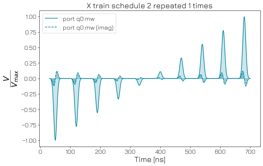
As you can see, the amplitude of the pulse (which was compiled from the X gate) changes.

Attention: A few device element parameter names do not correspond to the device_overrides key names. The integration_time of device elements can be overridden with the "acq_duration" key. These discrepancies are rare; in all cases the device element’s factory_kwargs must be used in the already generated compilation config.