See also
A Jupyter notebook version of this tutorial can be downloaded here.
Timetag acquisition tutorial#
The QTM enables us to detect pulses, by recording a TTL signal based on a settable analog threshold, that arrive at the input channels and to accurately timetag these detections to within 20 ps. The conversion of the detected signal to a timetag is arried out by a time to digital converter (referred to as TDC) inside of the QTM. In this tutorial, we will demonstrate this sequencer based timetagging operation.
There are three modes of operation one use the QTM to timetag incoming signals:
Scope Mode
This is the TTL-only counterpart to the scope acquisition of the analog QRM module.
When a scope acquisition is initiated, timetags are acquired until the acquisition window is closed or the scope memory is filled up (total of 2048 timetags).
Timetags windowed
Here incoming signals are detected within an acquisition window specified by Q1ASM. A digital event is recorded if the incoming signal passes a preset analog threshold.
For each acquisition window an event count and a timedelta is stored in a memory bin.
Timetagging in burst mode
The QTM boasts a TDC which acquires incoming signals at a rate of 20 MHz. In the default mode, oversampling by factor of x2 is enabled on the TDC meaning the sustained repetition rate for TTL detection is 44 ns.
If the oversampling is disabled, then this latency between tags can be reduced with the caveat that timetags are acquired in ‘bursts’ (up to a memory limit). This tutorial will demonstrate how to use this feature as well.
[1]:
from __future__ import annotations

from typing import TYPE_CHECKING, Callable

import matplotlib.pyplot as plt
import numpy as np
from qcodes.instrument import find_or_create_instrument

from qblox_instruments import Cluster, ClusterType

if TYPE_CHECKING:
    from qblox_instruments.qcodes_drivers.module import Module
Scan For Clusters#
We scan for the available devices connected via ethernet using the Plug & Play functionality of the Qblox Instruments package (see Plug & Play for more info).
!qblox-pnp list
[2]:
cluster_ip = "10.10.200.42"
cluster_name = "cluster0"
Connect to Cluster#
We now make a connection with the Cluster.
[3]:
cluster = find_or_create_instrument(
    Cluster,
    recreate=True,
    name=cluster_name,
    identifier=cluster_ip,
    dummy_cfg=(
        {
            2: ClusterType.CLUSTER_QCM,
            4: ClusterType.CLUSTER_QRM,
            6: ClusterType.CLUSTER_QCM_RF,
            8: ClusterType.CLUSTER_QRM_RF,
            10: ClusterType.CLUSTER_QTM,
        }
        if cluster_ip is None
        else None
    ),
)
Get connected modules#
[4]:
def get_connected_modules(cluster: Cluster, filter_fn: Callable | None = None) -> dict[int, Module]:
    def checked_filter_fn(mod: ClusterType) -> bool:
        if filter_fn is not None:
            return filter_fn(mod)
        return True

    return {
        mod.slot_idx: mod for mod in cluster.modules if mod.present() and checked_filter_fn(mod)
    }
[5]:
# QTM baseband modules
modules = get_connected_modules(cluster, lambda mod: mod.is_qtm_type)
[6]:
# This uses the module of the correct type with the lowest slot index
module = list(modules.values())[0]
Reset the Cluster#
We reset the Cluster to enter a well-defined state. Note that resetting will clear all stored parameters, so resetting between experiments is usually not desirable.
[7]:
cluster.reset()
print(cluster.get_system_status())
Status: OKAY, Flags: NONE, Slot flags: NONE
Timetag acquisition#
We will demonstrate the timetagging by sending digital pulses from one channel and acquiring these pulses from another channel.
In order to do so, we will open an acquisition window whose duration is fixed, and generate a sequence of pulses within this window. We define the opening time of the acquisition window as the reference time to date the pulses.
Define parameters#
Here we will set the parameters relevant to send digital signals from one of the QTM channels and acquire that signal from the QTM channel. We set the pulse number to the total number of timetags we wish to acquire.
Using the scope mode we are able to retrieve a maximum of 2048 timetags. In the scope mode, once the acquisition window is open, all the incoming detections are timetagged until the memory is full (2048 timetags) or until the user stops the acquisition.
[8]:
# Define the pulse duration for our output loop and the initial wait time.
PULSE_DURATION: int = 20  # ns
WAIT_TIME: int = 100  # ns
# Set the pulse number to the total number of timetags we wish to acquire.
PULSE_NUMBER: int = 20
# The threshold voltage that that a signal need to pass in order to be classed a detection event.
THRESHOLD: float = 0.5
# Acquisition duration in ns. Time for which the window will remain open.
ACQUISITION_DURATION: int = 2000  # ns
Configure QTM channels#
We first need to configure the QTM’s channels. The QTM has a one-to-one channel mapping between inputs and outputs of its eight sequencers. Configuring a channel is equivalent to configuring the sequencer with the same channel index.
Note
Each channel of the QTM can both work in output or input mode. Their indexing in the qblox_instruments API goes from Module.io_channel0 to Module.io_channel7, whereas the index label on the front panel of the module (this is what is referred to in the text above and throughout the script) goes from 1 to 8.
Here we will choose channel 5 from which to output digital pulses, with a wait time that is increased every 20 ns. These pulses will then be acquired by channel 1.
[9]:
# Synchronize the two sequencers that will be used.
module.sequencer0.sync_en(True)
module.sequencer4.sync_en(True)

# Enable the output channel to be controlled by the sequencer.
module.io_channel0.mode("output")

# Disable the output mode of the channel we want to acquire with, and set the threshold mode for detection.
module.io_channel4.mode("input")
module.io_channel4.analog_threshold(THRESHOLD)

# Set the time reference for time stamps to the start of the acquisition window.
module.io_channel4.binned_acq_time_ref("start")

# Record the time delta as 0 if no pulse is detected.
module.io_channel4.binned_acq_on_invalid_time_delta("record_0")

# Set the sequencer to trigger the scope mode.
module.io_channel4.scope_trigger_mode("sequencer")

# Set the scope mode to acquire all timetags.
module.io_channel4.scope_mode("timetags")
Define a program for the output of digital pulses.
[10]:
program_pulse = f"""
    move            {WAIT_TIME}, R0
    move            {PULSE_NUMBER}, R1
    wait_sync       4

    loop:
        set_digital 1,1,0  # level (1=high), mask (always 1 for v1), fine_delay in steps of 1/128 ns
        upd_param   4
        wait        {PULSE_DURATION - 4}
        set_digital 0,1,0
        upd_param   4
        wait        R0

        add         R0,1000, R0
        nop
        loop        R1, @loop
    stop
"""
Define a program for the acquisition of timetags.
[11]:
program_acq = f"""
    move        0, R0
    move        0, R2
    wait_sync   4

    set_scope_en 1

    set_time_ref
    acquire_timetags 0, R0, 1, R2, 4 # fine_delay steps of 1/128 ns, 5 steps = 39 ps
    wait             {ACQUISITION_DURATION}
    acquire_timetags 0, R0, 0, R2, 4

    stop
"""
Create an acquisition dictionary to store timetags and upload the programs to the appropriate sequencer.
[12]:
# Define acquisition dictionary.
acquisition_modes: dict[str, dict[str, int]] = {
    "timetag_single": {"num_bins": 1, "index": 0},
    "timetag_fully_binned": {"num_bins": 131_072, "index": 1},
}
# Upload the pulse program to the sequencer.
module.sequencer0.sequence(
    {
        "waveforms": {},
        "weights": {},
        "acquisitions": {},
        "program": program_pulse,
    }
)
# Upload the acquisitions and program to the sequencer.
module.sequencer4.sequence(
    {
        "waveforms": {},
        "weights": {},
        "acquisitions": acquisition_modes,
        "program": program_acq,
    }
)

module.sequencer0.arm_sequencer()
module.sequencer4.arm_sequencer()
[13]:
# Start sequencer.
module.start_sequencer()
[14]:
# Check sequencer status.
print(module.get_sequencer_status(0))
print(module.get_sequencer_status(4))

# Wait for the acquisition to finish with a timeout period of one minute.
module.get_acquisition_status(4, 1)

# Move acquisition data from temporary memory to acquisition list.
scope_data = module.io_channel4.get_scope_data()
scope_data = (
    scope_data if scope_data else np.zeros((2, 100))
)  # dummy data if the dummy cluster is used
Status: OKAY, State: STOPPED, Info Flags: NONE, Warning Flags: NONE, Error Flags: NONE, Log: []
Status: OKAY, State: STOPPED, Info Flags: ACQ_BINNING_DONE, Warning Flags: NONE, Error Flags: NONE, Log: []
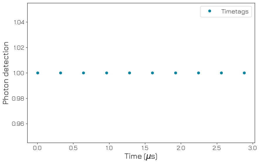
The absolute timetags are expressed in units of (1/2048) ns relative to the CTC (internal clock) of the module. This means we must convert the acquired timetags to the appropriate units relative to the timetag of the first event in the trace.
[15]:
print(f"Number of acquired timetags in window: {len(scope_data)}")
# Convert the acquired timetags to the correct units.
timetags = np.array([(i[1] - scope_data[0][1]) / (2048e3) for i in scope_data])

fig, ax = plt.subplots(1, 1)
ax.plot(timetags, np.ones(len(timetags)), "o", label="Timetags")
ax.set_xlabel(r"Time ($\mu$s)")
ax.set_ylabel("Photon detection")
plt.legend(loc="upper right")
plt.show()
Number of acquired timetags in window: 20
Windowed scope timetag acquisition#
We will now repeat the scope measurement we carried out above by specifying a window and activating the ‘windowed scope’ mode such that the timetags are only acquired in certain time window. The size of the scope acquisition window is determined by the duration for which the acquire timetags window is kept open in the Q1ASM program.
[16]:
# Set the scope mode to acquire timetags in a certain window for the acquisition channel.
module.io_channel4.scope_mode("timetags-windowed")

# Set the acquisition duration.
ACQUISITION_DURATION: int = 5000
[17]:
# Define acquisition program.
program_acq = f"""
    move        0, R0
    move        0, R2
    wait_sync   4

    set_scope_en 1
    set_time_ref
    acquire_timetags 0, R0, 1, R2, 4 # fine_delay steps of 1/128 ns, 5 steps = 39 ps
    wait             {ACQUISITION_DURATION}
    acquire_timetags 0, R0, 0, R2, 4
    stop
"""
[18]:
# Upload the pulse program to the sequencer.
module.sequencer0.sequence(
    {
        "waveforms": {},
        "weights": {},
        "acquisitions": {},
        "program": program_pulse,
    }
)

# Upload the acquisitions program to the sequencer.
module.sequencer4.sequence(
    {
        "waveforms": {},
        "weights": {},
        "acquisitions": acquisition_modes,
        "program": program_acq,
    }
)
[19]:
# Arm sequencers.
module.sequencer0.arm_sequencer()
module.sequencer4.arm_sequencer()
[20]:
# Start sequencers.
module.start_sequencer()
[21]:
# Check sequencer status.
print(module.get_sequencer_status(0))
print(module.get_sequencer_status(4))

# Wait for the acquisition to finish with a timeout period of one minute.
module.get_acquisition_status(4, 1)
# Extract scope data.
scope_data = module.io_channel1.get_scope_data()
scope_data = (
    scope_data if scope_data else np.zeros((2, 100))
)  # dummy data if the dummy cluster is used
Status: OKAY, State: STOPPED, Info Flags: NONE, Warning Flags: NONE, Error Flags: NONE, Log: []
Status: OKAY, State: STOPPED, Info Flags: ACQ_BINNING_DONE, FORCED_STOP, Warning Flags: NONE, Error Flags: NONE, Log: []
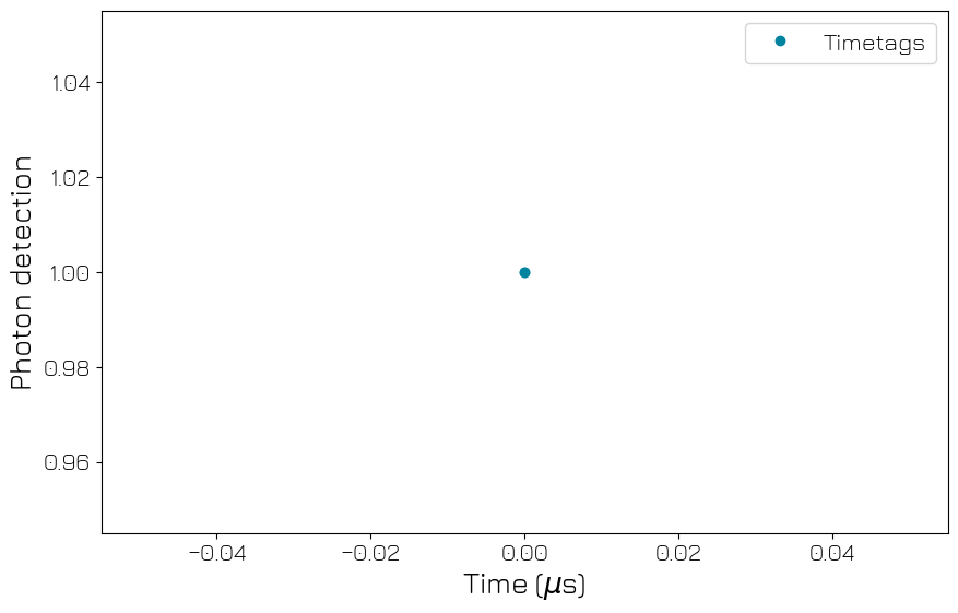
[22]:
print(f"Number of acquired timetags in window: {len(scope_data)}")

# Convert the units of timetags to us.
timetags = np.array([(i[1] - scope_data[0][1]) / (2048e3) for i in scope_data])  # in us

fig, ax = plt.subplots(1, 1)
ax.plot(timetags, np.ones(len(timetags)), "o", label="Timetags")
ax.set_xlabel(r"Time ($\mu$s)")
ax.set_ylabel("Photon detection")
plt.legend(loc="upper right")
plt.show()
Number of acquired timetags in window: 2
Binned Timetag Acquisition#
Here we utilize trigger based acquisition to efficiently capture every single pulse arriving at the QTM and store the resultant timedelta in a bin.
This demonstration will allow us to circumvent the memory limit of the scope mode (limited to 2048 timetags), by opening and closing an acquisition window based on a trigger, which is the event detection itself. In this case, the memory limit for the number of saved events is 131072, which corresponds to the number of bins available with each sequencer.
Even though this approach allows to store more timetags, it is important to note that the time resolution of the timetags is now set by the duration of the acquisition (corresponding to a bin) which will typically be much larger than the intrinsic resolution of the QTM (39ps). This is due to an inherent trade-off between being able acquire high flux signals and being able to accurately timetag them all with high precision.
To enable trigger-based closing of the acquisition window, we need to make sure that the typical duration between two events in the signal is much greater than 252 ns, which represents the latency in our trigger network. In case a trigger is sent to the trigger network less than 252 ns after the previous one, it will be missed, and a warning flag will be raised in the sequencer forwarding the trigger.
[23]:
# Define some parameters for the binned acquisition.
ACQ_REPS: int = 131072  # Number of bins, i.e timetags to acquire
WAIT_TIME: int = 300  # ns

module.io_channel4.mode("input")
module.io_channel4.analog_threshold(THRESHOLD)

# Set up channel 1 to send a trigger on the trigger network with trigger address=1 everytime it detects an event.
module.io_channel4.forward_trigger_en(True)
module.io_channel4.forward_trigger_mode("rising")
module.io_channel4.forward_trigger_address(1)

# Set the reference to which all timetags are measured. The time reference is configured through a
# Q1ASM instruction.
# We also configure the time source to be 'first', meaning the timetag from the first detection will be used.
module.io_channel4.binned_acq_time_ref("sequencer")
module.io_channel4.binned_acq_time_source("first")
module.io_channel4.binned_acq_on_invalid_time_delta("record_0")
Define programs for sending and acquiring pulses.
[24]:
# Program to output digital pulses.
program_pulse = f"""
    move            {WAIT_TIME}, R0
    move            {ACQ_REPS}, R1
    wait_sync       4

    loop:
        set_digital 1,1,0  # level (1=high), mask (always 1 for v1), fine_delay in steps of 1/128 ns
        upd_param   4
        wait        {PULSE_DURATION - 4}
        set_digital 0,1,0
        upd_param   4
        wait        {WAIT_TIME - 4}
        loop        R1, @loop
    stop
"""
[25]:
# Program to acquire timetags.
program_bin = f"""
    move            0, R0
    move            {ACQ_REPS},R1
    move            0, R2

    set_scope_en    1
    wait_sync       4
    set_time_ref
    loop:
        acquire_timetags 1, R0, 1, R2, 4
        wait_trigger     1, 4
        acquire_timetags 1, R0, 0, R2, 4
        add              R0, 1, R0
        nop
        loop             R1, @loop   #Repeat loop until R1 is 0
    stop
"""
[26]:
# Upload the pulse program to the sequencer
module.sequencer0.sequence(
    {
        "waveforms": {},
        "weights": {},
        "acquisitions": {},
        "program": program_pulse,
    }
)

# Upload the acquisitions and program to the sequencer
module.sequencer4.sequence(
    {
        "waveforms": {},
        "weights": {},
        "acquisitions": acquisition_modes,
        "program": program_bin,
    }
)
[27]:
# Arm sequencers.
module.arm_sequencer(0)
module.arm_sequencer(4)
[28]:
# Start sequencer.
module.start_sequencer()
[29]:
# Print status of sequencer.
print(module.get_sequencer_status(0))
print(module.get_sequencer_status(4))
Status: OKAY, State: RUNNING, Info Flags: FORCED_STOP, Warning Flags: NONE, Error Flags: NONE, Log: []
Status: OKAY, State: RUNNING, Info Flags: FORCED_STOP, Warning Flags: NONE, Error Flags: NONE, Log: []
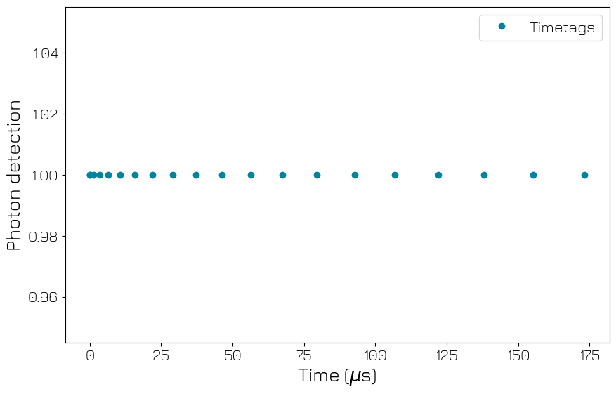
Here we plot the extracted timetags and the photon count associated with each bin. For each acquisition window, a photon count (sum of all detections in that window) and one timedelta (the difference between the measured timetag and reference) are stored in a corresponding bin.
[30]:
# Wait for the acquisition to finish with a timeout period of one minute.
module.get_acquisition_status(4, 1)
# Extract the acquisition from the sequencer.
acq = module.get_acquisitions(4)
[31]:
photon_count = acq["timetag_fully_binned"]["acquisition"]["bins"]["count"]
timetags = acq["timetag_fully_binned"]["acquisition"]["bins"]["timedelta"]
photon_count = (
    photon_count if not np.any(np.isnan(photon_count)) else np.zeros(100)
)  # dummy data if the dummy cluster is used
Below we plot the first 10 acquired timetags to check their timestamps are correct.
[32]:
# Here we plot the acquired timetags for the acquisitions that we carried out.
timetags = [i / (2048e3) for i in timetags]  # in us

fig, ax = plt.subplots(1, 1)
ax.plot(timetags[:10], np.ones(len(timetags))[:10], "o", label="Timetags")
ax.set_xlabel(r"Time ($\mu$s)")
ax.set_ylabel("Photon detection")
plt.legend(loc="upper right")
plt.show()
Verify that the sum of the photon counts in each bin corresponds to the number of pulses sent.
[33]:
# Here we plot the acquired photon counts from each bin in the form of a histogram.
# We see indeed that we only ever count 1 photon during each acquisition.
plt.hist(photon_count)
plt.ylabel("Occurrences")
plt.xlabel("Detected photons")
plt.show()

# Total number of detections in the measurement is found by summing the photon count in all the bins.
print(f"The total photon count is {np.sum(photon_count)}")
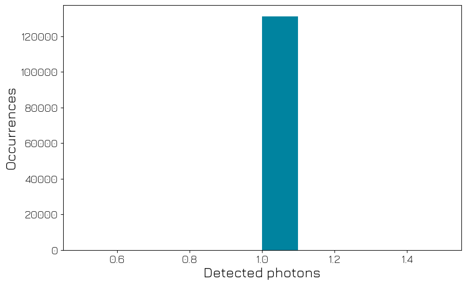
The total photon count is 131072.0
Low-latency burst mode#
The TDC inside the QTM has an internal buffer of 16 entries and can send detection events to the FPGA at a rate of 44 ns per timetags. This creates a total latency of 704 ns, or the total time for available for the TDC to buffer timetags.
If the oversampling of the TDC is disabled, any pulse sequences arriving at the QTM faster than a period of 44 ns will be handled correctly. This means the QTM can timetag with a lower latency (with a limit of 20 ns) until the total time buffer is filled up.
Here we will repeat the initial scope acquisition, except we will acquire a signal with a click rate faster than the 44 ns latency limit of the QTM. .. note:: The QTM can acquire timetags at this reduced latency, but only in short bursts that are determine by the buffer memory of the TDC module inside.
Setting up the QTM to perform low latency time-tagging#
[34]:
# Reset the cluster before we begin this measurement scheme.
cluster.reset()
print(cluster.get_system_status())
Status: OKAY, Flags: NONE, Slot flags: NONE
Here we disable the oversampling of the TDC in both quads of the QTM which will enable us to carry out a burst measurement.
[35]:
# The channels in the QTM are grouped into two quads with four channels, that are indexed as
# 0 and 1 respectively.
# The TDC oversampling can be disabled at the quad level using the following command.
module.quad0.timetag_oversampling("disabled")
module.quad1.timetag_oversampling("disabled")
Here we configure the two channels again to acquire signals in windowed scope mode.
[36]:
# Synchronize the sequencers that will be used.
module.sequencer0.sync_en(True)
module.sequencer4.sync_en(True)
[37]:
# Enable the output channel to be controlled by the sequencer
module.io_channel0.mode("output")
Configure the input channel#
[38]:
# Disable the output mode of the channel we want to acquire with, and set the threshold
# mode for detection.
module.io_channel4.mode("input")
module.io_channel4.analog_threshold(THRESHOLD)

# Set qcodes parameters for acquiring signals
module.io_channel4.binned_acq_time_ref("start")
module.io_channel4.binned_acq_on_invalid_time_delta("record_0")
module.io_channel4.scope_trigger_mode("sequencer")

module.io_channel4.scope_mode("timetags-windowed")
[39]:
PULSE_DURATION: int = 10  # ns
WAIT_TIME: int = 10  # ns
We will now define a Q1ASM program to produce a series of TTL pulses that arrive with a higher frequency. In this case we have set the wait time to be 10 ns and the pulse duration to be 10 ns. This results in the spacing between successive rising edges to be 20 ns, which is well below the 44 ns latency limit.
We will transmit 24 pulses, which we hope to timetag with 20 ps precision, demonstrating the low latency burst mode.
[40]:
# Define parameter that determines the number of pulses.
NUM_PULSE: int = 24
[41]:
program_pulse_high_rate = f"""

    move                {WAIT_TIME}, R0
    move                {NUM_PULSE}, R1
    wait_sync           4

    loop:

        set_digital     1,1,0               # level (1=high), mask (always 1 for v1), fine_delay in steps of 1/128 ns
        upd_param       {PULSE_DURATION}
        set_digital     0,1,0

        upd_param       {WAIT_TIME}
        loop            R1, @loop
    stop
"""
We will use the same acquisition program as before, and trigger a windowed scope acquisition.
[42]:
ACQUISITION_DURATION: int = 1000 # ns
[43]:
# Define acquisition program.
program_acq = f"""
    move        0, R0
    move        0, R2
    wait_sync   4

    set_scope_en 1
    set_time_ref
    acquire_timetags 0, R0, 1, R2, 4 # fine_delay steps of 1/128 ns, 5 steps = 39 ps
    wait             {ACQUISITION_DURATION}
    acquire_timetags 0, R0, 0, R2, 4

    stop
"""
[44]:
# Define acquisition dictionary.
acquisition_modes: dict[str, dict[str, int]] = {"timetag_single": {"num_bins": 1, "index": 0}}
[45]:
# Upload the pulse program to the sequencer.
module.sequencer0.sequence(
    {
        "waveforms": {},
        "weights": {},
        "acquisitions": {},
        "program": program_pulse_high_rate,
    }
)

# Upload the acquisitions program to the sequencer.
module.sequencer4.sequence(
    {
        "waveforms": {},
        "weights": {},
        "acquisitions": acquisition_modes,
        "program": program_acq,
    }
)
[46]:
module.sequencer0.arm_sequencer()
module.sequencer4.arm_sequencer()
[47]:
module.start_sequencer()
[48]:
# Check sequencer status.
print(module.get_sequencer_status(0))
print(module.get_sequencer_status(4))
Status: OKAY, State: STOPPED, Info Flags: NONE, Warning Flags: NONE, Error Flags: NONE, Log: []
Status: OKAY, State: STOPPED, Info Flags: ACQ_BINNING_DONE, Warning Flags: NONE, Error Flags: NONE, Log: []
[49]:
# Wait for the acquisition to finish with a timeout period of one minute.
print(module.get_acquisition_status(4, 1))
# Extract scope data.
scope_data = module.io_channel4.get_scope_data()
scope_data = (
    scope_data if scope_data else np.zeros((2, 100))
)  # dummy data if the dummy cluster is used
True
[50]:
print(f"Number of acquired timetags in window: {len(scope_data)}")

# Convert the units of timetags to us.
timetags = np.array([(i[1] - scope_data[0][1]) / (2048) for i in scope_data])  # in ns
Number of acquired timetags in window: 26
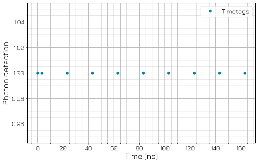
The acquired timetags of the high frequency signal are displayed below.
[51]:
timetags_to_plot = timetags[0:10]

fig, ax = plt.subplots(1, 1)
ax.plot(timetags_to_plot, np.ones(len(timetags_to_plot)), "o", label="Timetags")
ax.set_xlabel("Time (ns)")
ax.set_ylabel("Photon detection")
plt.legend(loc="upper right")
plt.grid(which="minor", linewidth=0.6)
plt.grid(which="major", linewidth=1.2)
plt.minorticks_on()
plt.show()