QCM demo
In this demo we showcase the upload and continuous play of waveform primitives using the Qblox Pulsar QCM. In addition we observe the output on a oscilloscope.
NB: This hardware demo interacts with firmware low-level interfaces. When building applications we highly recommend using Quantify framework.
# Set up environment
import os
import scipy.signal
import math
import json
import time
Connect to the QCM
# Add Pulsar QCM interface
from pulsar_qcm.pulsar_qcm import pulsar_qcm
# Connect to device over Ethernet
pulsar = pulsar_qcm("qcm", "192.168.0.2")
Tip
If you need to re-instantiate the instrument without re-starting
the Jupyter Notebook (or the ipython shell) run the following command first pulsar.close(). This closes the QCoDeS instrument instance.
# Print device information
print(pulsar.get_idn())
# Get system status
print(pulsar.get_system_status())
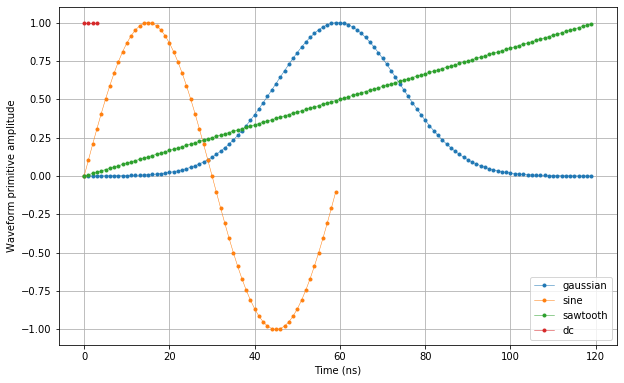
Generate waveforms for QCM
# Generate waveforms

waveform_len = 120  # ns

# "index" is used to select the waveforms at the hardware level
waveforms    = {
                 "gaussian": {"data": [], "index": 0},
                 "sine":     {"data": [], "index": 1},
                 "sawtooth": {"data": [], "index": 2},
                 "dc":       {"data": [], "index": 3}
               }

#Create gaussian waveform
if "gaussian" in waveforms:
    waveforms["gaussian"]["data"] = scipy.signal.gaussian(waveform_len, std=0.12 * waveform_len)

#Create gaussian waveform
if "sine" in waveforms:
    waveforms["sine"]["data"] = [math.sin((2 * math.pi / (0.5 * waveform_len)) * i ) for i in range(0, waveform_len//2)]

#Create sawtooth waveform
if "sawtooth" in waveforms:
    waveforms["sawtooth"]["data"] = [(1.0 / (waveform_len)) * i for i in range(0, waveform_len)]

#Create block waveform
if "dc" in waveforms:
    # NB for DC we only need to generate 4 sample points and play them on repeat
    waveforms["dc"]["data"] = [1.0 for i in range(0, 4)]
import matplotlib.pyplot as plt
import numpy as np

time = np.arange(0, max(map(lambda d: len(d["data"]), waveforms.values())), 1)

fig, ax = plt.subplots(1,1, figsize=(10, 10/1.61))

ax.set_ylabel("Waveform primitive amplitude")
ax.set_xlabel("Time (ns)")

for wf, d in waveforms.items():
    ax.plot(time[:len(d["data"])], d["data"], ".-", linewidth=0.5, label=wf)

ax.legend(loc=4)
ax.yaxis.grid()
ax.xaxis.grid()

In order to play the waveform the firmware needs to receive the waveforms as well as an assembly-like program. In this case we will be running the device in continuous mode, i.e. the same waveforms will be played over and over again on the same outputs. This makes easy to get started and observe the waveforms on an oscilloscope and the required program is trivial.
Currently, the output pair \(\mathrm{O}^1\) & \(\mathrm{O}^2\) is controlled by its own CPU-like sequence processor (sequencer); and similarly for \(\mathrm{O}^3\) & \(\mathrm{O}^4\). This will become much more flexible with new firmware and software updates.
Note
Currently, playing waveforms in continuous mode requires the number of samples of the waveforms to be multiples of 4.
Generate program and waveforms file for QCM
We are going to play waveforms in continuous mode. Since this requites bypassing the sequence processor’s control over the waveform memory to directly play the waveforms in a continuous repeated mode the sequencer processors needs to stop immediately when started, therefore the only instruction necessary in the program is a stop instruction.
Note
For more elaborated experiments there will be an assembly-like program file for each sequencer generated by a compiler from a higher level interface.
# Sequencer programs
seq_prog = ["stop", "stop"]
# Write waveforms and programs to a JSON files
for name in waveforms:
    if str(type(waveforms[name]["data"]).__name__) == "ndarray":
        assert (len(waveforms[name]["data"]) % 4) == 0,\
                "In continuous waveform mode the lenght of a waveform must be a mupltiple of 4!"

        waveforms[name]["data"] = waveforms[name]["data"].tolist()  # JSON only supports lists

for seq, prog in enumerate(seq_prog):
    wave_and_prog_dict = {"waveforms": {"awg": waveforms},
                          "program": prog}
    with open("demo_seq{}.json".format(seq), 'w', encoding='utf-8') as file:
        json.dump(wave_and_prog_dict, file, indent=4)
        file.close()
Upload program and waveforms into QCM
# Upload waveforms and programs
for seq in [0, 1]:
    pulsar.set(
        "sequencer{}_waveforms_and_program".format(seq),
        os.path.join(os.getcwd(), "demo_seq{}.json".format(seq))
    )
    print(pulsar.get_assembler_log())
Configure the QCM
# Configure the sequencers
for seq in [0, 1]:
    pulsar.set("sequencer{}_sync_en".format(seq),                 True)  # Enable the sequecer
    pulsar.set("sequencer{}_cont_mode_en_awg_path0".format(seq),  True)  # Set continuous waveform repetition on O1/O3 outputs
    pulsar.set("sequencer{}_cont_mode_en_awg_path1".format(seq),  True)  # Set continuous waveform repetition on O2/O4 outputs
    pulsar.set("sequencer{}_gain_awg_path0".format(seq),          1.0)   # Set unitary gain on O1/O3 outputs
    pulsar.set("sequencer{}_gain_awg_path1".format(seq),          1.0)   # Set unitary gain on O2/O4 outputs
    pulsar.set("sequencer{}_offset_awg_path0".format(seq),        0)     # No offsets on O1/O3 outputs
    pulsar.set("sequencer{}_offset_awg_path1".format(seq),        0)     # No offsets on O2/O4 outputs
    pulsar.set("sequencer{}_mod_en_awg".format(seq),              False) # Disable modulation

# Which waveform on which output?
pulsar.set("sequencer0_cont_mode_waveform_idx_awg_path0".format(seq), 0) # Gaussian on O1
pulsar.set("sequencer0_cont_mode_waveform_idx_awg_path1".format(seq), 1) # Sine on O2
pulsar.set("sequencer1_cont_mode_waveform_idx_awg_path0".format(seq), 2) # Sawtooth on 03
pulsar.set("sequencer1_cont_mode_waveform_idx_awg_path1".format(seq), 3) # DC on O4
Play waveforms on the QCM
# Arm the sequencers
pulsar.arm_sequencer()
# Start the sequencers
pulsar.start_sequencer()

# Print status
for seq in range(0, 2):
    print(pulsar.get_sequencer_state(seq))
Visualize the signals on an oscilloscope
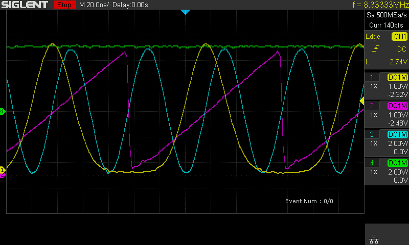
We connect all output channels of the QCM to the four channels of an oscilloscope. On the scope we are able to see that all waveforms are being generated correctly:

# Stop the sequencers
pulsar.stop_sequencer()
for seq in range(0, 2):
    print(pulsar.get_sequencer_state(seq))
# It is also possible to retrieve back the waveforms in the memory
wvs = pulsar.get_waveforms(0)["awg"]

import matplotlib.pyplot as plt

time = np.arange(0, max(map(lambda d: len(d["data"]), wvs.values())), 1)

fig, ax = plt.subplots(1,1, figsize=(10, 10/1.61))

ax.set_ylabel("Waveform primitive amplitude")
ax.set_xlabel("Time (ns)")

for wf, d in wvs.items():
    ax.plot(time[:len(d["data"])], d["data"], ".-", linewidth=0.5, label=wf)

ax.legend(loc=4)
ax.yaxis.grid()
ax.xaxis.grid()

Since we are using a QCoDeS interface for our instrument we can retrieve an overview of its parameters:
# Print the instrument snapshot
# See QCoDeS documentation for details
pulsar.print_readable_snapshot(update=True)