See also
A Jupyter notebook version of this tutorial can be downloaded here.
Rabi experiment#
In this tutorial we will combine the techniques explained in the other tutorials and show how to perform a Rabi experiment. For this tutorial we will need one QCM to generate the Rabi pulses and one QRM to perform the readout, although the QCM could be replaced by another QRM if needed.
Ports \(\text{O}^{[1-2]}\) of the QCM are used for the driving pulse, while \(\text{O}^{[1-2]}\) of the QRM are used for the readout pulse. Finally, ports \(\text{I}^{[1-2]}\) are used for the acquisition of the readout tone. In this tutorial it is assumed \(\text{O}^{1}\) of the QRM is connected to \(\text{I}^{1}\) of the QRM for time of flight calibration. Furthermore we assume that \(\text{O}^{1}\) of the QCM and \(\text{O}^{2}\) of the QRM are connected to an external oscilloscope to view the Rabi experiment pattern. The scope can be triggered of marker 1 of the QCM.
As demonstrated in the synchronization tutorial, the SYNQ technology synchronizes the programs in the two modules. If you are using Pulsar modules, to ensure synchronization between the modules, connect the \(\text{REF}^{out}\) of the Pulsar QCM to the \(\text{REF}^{in}\) of the Pulsar QRM using a coaxial cable, and connect their SYNQ ports using the SYNQ cable.
If you are using a Cluster, then no extra connection needs to be made as the modules are internally connected with SYNQ capability.
To run this tutorial please make sure you have installed and enabled ipywidgets:
pip install ipywidgets
jupyter nbextension enable --py widgetsnbextension
Setup#
First, we are going to import the required packages and connect to the instrument.
[1]:
# Import ipython widgets
import contextlib
import json

import ipywidgets as widgets
import matplotlib.pyplot as plt
import numpy as np

# Set up the environment.
from IPython.display import display
from qcodes import Instrument

from qblox_instruments import Cluster, PlugAndPlay, Pulsar
Scan For Clusters#
We scan for the available devices connected via ethernet using the Plug & Play functionality of the Qblox Instruments package (see Plug & Play for more info).
[2]:
!qblox-pnp list
Devices:
 - 10.10.200.42: cluster_mm 0.6.1 with name "QAE_1" and serial number 00015_2320_004
 - 10.10.200.50: cluster_mm 0.6.1 with name "cluster-mm" and serial number 00015_2219_003
 - 10.10.200.51: pulsar_qcm 0.11.1 with name "pulsar-qcm" and serial number 00012_2039_005
 - 10.10.200.52: pulsar_qrm 0.11.1 with name "pulsar-qrm" and serial number 00013_2120_008
 - 10.10.200.53: cluster_mm 0.6.1 with name "cluster-mm" and serial number 00015_2320_003
[3]:
cluster_ip = "10.10.200.42"
cluster_name = "cluster0"
Connect to Cluster#
We now make a connection with the Cluster.
[4]:
from qblox_instruments import Cluster, ClusterType

try:  # Close the chosen QCodes instrument to prevent name clash
    Cluster.find_instrument(cluster_name).close()
except KeyError:
    pass

cluster = Cluster(
    name=cluster_name,
    identifier=cluster_ip,
    dummy_cfg={
        2: ClusterType.CLUSTER_QCM,
        4: ClusterType.CLUSTER_QRM,
        6: ClusterType.CLUSTER_QCM_RF,
        8: ClusterType.CLUSTER_QRM_RF,
    }
    if cluster_ip is None
    else None,
)
Get connected modules#
[5]:
def get_connected_modules(cluster, filter_fn=None):
    def checked_filter_fn(mod):
        if filter_fn is not None:
            return filter_fn(mod)
        return True

    return {
        mod.slot_idx: mod for mod in cluster.modules if mod.present() and checked_filter_fn(mod)
    }
[6]:
# QRM baseband modules
readout_modules = get_connected_modules(cluster, lambda mod: mod.is_qrm_type and not mod.is_rf_type)
readout_modules
[6]:
{4: <QcmQrm: cluster0_module4 of Cluster: cluster0>}
[7]:
readout_module = readout_modules[4]
[8]:
# QCM baseband modules
control_modules = get_connected_modules(
    cluster, lambda mod: not mod.is_qrm_type and not mod.is_rf_type
)
control_modules
[8]:
{2: <QcmQrm: cluster0_module2 of Cluster: cluster0>}
[9]:
control_module = control_modules[2]
Sequencer Setup#
Set sync_en to synchronize across modules.
[10]:
# Set sync_en
readout_module.sequencer0.sync_en(True)
control_module.sequencer0.sync_en(True)
Configure the NCO of both the QRM and QCM to 100 MHz and enable the up- and down-conversion in the sequencers
[11]:
readout_module.sequencer0.nco_freq(100e6)
readout_module.sequencer0.mod_en_awg(True)
readout_module.sequencer0.demod_en_acq(True)

control_module.sequencer0.nco_freq(100e6)
control_module.sequencer0.mod_en_awg(True)
Configure the outputs of the QRM and QCM such that sequencer0 is the only enabled sequencer and maps to \(\text{O}^{[1-2]}\)
[12]:
# Map sequencer of the QCM to specific outputs (but first disable all sequencer connections)
control_module.disconnect_outputs()

control_module.sequencer0.connect_sequencer("out0_1")

# Map sequencer of the QRM to specific outputs (but first disable all sequencer connections)
readout_module.disconnect_outputs()
readout_module.disconnect_inputs()

readout_module.sequencer0.connect_sequencer("io0_1")
Define waveforms#
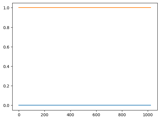
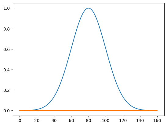
To readout the systems we define constant pulses one and zero which will be up converted by the NCO to create the appropriate tones for an IQ mixer. Similarly for driving the qubit, we define a Gaussian pulse, together with a zero pulse of equal length to serve as inputs for an IQ mixer. In this tutorial we do not assume mixers to be connected to the inputs and outputs of the QCM/QRM.
[13]:
t = np.arange(-80, 81, 1)
sigma = 20
wfs = {
    "zero": {"index": 0, "data": [0.0] * 1024},
    "one": {"index": 1, "data": [1.0] * 1024},
    "gauss": {"index": 2, "data": list(np.exp(-(0.5 * t**2 / sigma**2)))},
    "empty": {"index": 3, "data": list(0.0 * t)},
}
Hence we obtain the following waveforms for readout:
[14]:
plt.plot(wfs["zero"]["data"])
plt.plot(wfs["one"]["data"])
[14]:
[<matplotlib.lines.Line2D at 0x19cfee54fd0>]

And for drive:
[15]:
plt.plot(wfs["gauss"]["data"])
plt.plot(wfs["empty"]["data"])
[15]:
[<matplotlib.lines.Line2D at 0x19c82074700>]

Finally, we define two acquisitions. A single readout to perform the calibration measurements. Secondly we create a rabi readout sequence that contains 50 different bins for saving the results, one for each of the different amplitudes used for the drive tone.
[16]:
num_bins = 50  # Number of amplitudes to be measured
acquisitions = {
    "single": {"num_bins": 1, "index": 0},
    "rabi": {"num_bins": num_bins, "index": 1},
}
Calibration experiments#
TOF calibration#
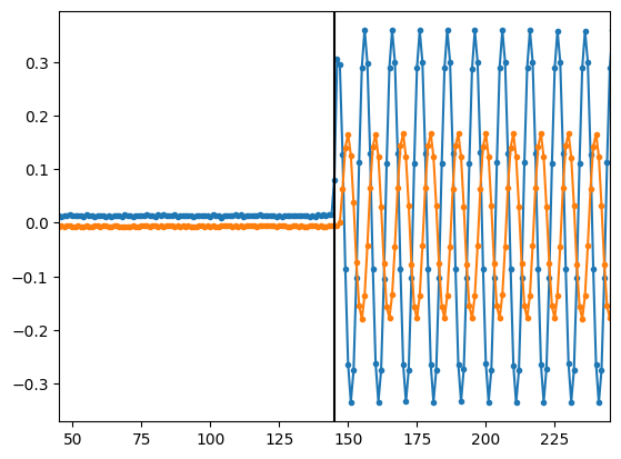
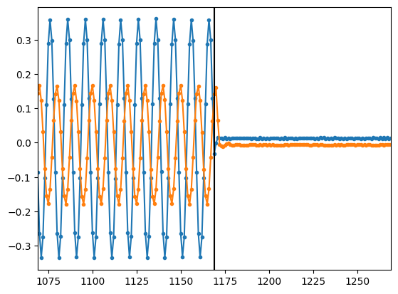
As a first step, we calibrate the time of flight (tof) for the QRM module. In order to do so, we play a readout pulse and analyze the obtained signal on the oscilloscope to find the travel time of the pulse through the system.
[17]:
qrm_prog = """
play    1, 0, 4     # start readout pulse
acquire 0, 0, 16384 # start the 'single' acquisition sequence and wait for the length of the scope acquisition window
stop
"""
Upload the program, together with the waveforms and acquisitions to the QRM
[18]:
sequence = {
    "waveforms": wfs,
    "weights": {},
    "acquisitions": acquisitions,
    "program": qrm_prog,
}
with open("sequence.json", "w", encoding="utf-8") as file:
    json.dump(sequence, file, indent=4)
    file.close()
# Upload sequence.
readout_module.sequencer0.sequence("sequence.json")
Perform the calibration experiment
[19]:
# Arm and start sequencer.
readout_module.arm_sequencer(0)
readout_module.start_sequencer()

# Wait for the sequencer and acquisition to finish with a timeout period of one minute.
readout_module.get_acquisition_state(0, 1)
readout_module.store_scope_acquisition(0, "single")
# Print status of sequencer.
print(readout_module.get_sequencer_state(0))
Status: STOPPED, Flags: FORCED_STOP, ACQ_SCOPE_DONE_PATH_0, ACQ_SCOPE_DONE_PATH_1, ACQ_BINNING_DONE
Analyze the resulting signal on the scope to find the tof
[20]:
p0 = np.array(readout_module.get_acquisitions(0)["single"]["acquisition"]["scope"]["path0"]["data"])
p1 = np.array(readout_module.get_acquisitions(0)["single"]["acquisition"]["scope"]["path1"]["data"])
# Determine when the signal crosses half-max for the first time (in ns)
t_halfmax = np.where(np.abs(p0) > np.max(p0) / 2)[0][0]

# The time it takes for a sine wave to reach its half-max value is (in ns)
correction = 1 / readout_module.sequencer0.nco_freq() * 1e9 / 12

tof_measured = t_halfmax - correction
Plot the signal on the scope, around the rising and falling edge of the acquisition signal, as determined by the tof analysis above:
[21]:
r = readout_module.get_acquisitions(0)["single"]["acquisition"]["scope"]
plt.plot(r["path0"]["data"], ".-")
plt.plot(r["path1"]["data"], ".-")
plt.axvline(tof_measured, c="k")
plt.xlim(
    tof_measured - 10 / readout_module.sequencer0.nco_freq() * 1e9,
    tof_measured + 10 / readout_module.sequencer0.nco_freq() * 1e9,
)
plt.show()

plt.plot(r["path0"]["data"], ".-")
plt.plot(r["path1"]["data"], ".-")
plt.axvline(1024 + tof_measured, c="k")
plt.xlim(
    1024 + tof_measured - 10 / readout_module.sequencer0.nco_freq() * 1e9,
    1024 + tof_measured + 10 / readout_module.sequencer0.nco_freq() * 1e9,
)
plt.show()


Parameters#
Set the parameters for the Rabi experiment
[22]:
# all times must be divisible by 4
reset_time = 200  # reset time for the qubit in microseconds
tof = int(tof_measured / 4) * 4  # time of flight must be divisible by 4
readout_delay = 164  # time to delay the readout pulse after the start of the rotation pulse

navg = 1000  # number of averages
stepsize = int(65535 / 100)
Rabi#
Normally, a Rabi experiment would be performed by changing the amplitude in the inner loop, and averaging in the outer loop. To make the resulting experiment visible on an oscilloscope however, in this tutorial we swapped these two loops
[23]:
# QCM sequence program.
qcm_seq_prog = f"""
# Registers used:
# R0 loops over the different awg amplitudes used for the rabi driving pulse
# R2 is used to count the averages needed for a single amplitude
# R3 contains the qubit reset time in microseconds

           move          0, R0                       # start with awg amplitude 0
           wait_sync     4                           # Synchronize the QRM with the QCM


ampl_loop: add           R0, {stepsize}, R0          # increase the pulse amplitude by the stepsize
           move          {navg}, R2                  # reset the number of averages and save in the R2 register

           # let the qubit relax to its groundstate
navg_loop: move          {reset_time}, R3            # reset the number of microseconds to wait and save in the R3 register
rst_loop:  wait          1000                        # wait 1 microsecond
           loop          R3,@rst_loop                # repeat the 1 microsecond wait as much as needed to let the qubit relax

           set_awg_gain  R0, R0                      # Set the new amplitude used for the drive pulse
           set_mrk       1                           # Set marker 1 high for to enable synchronization with external oscilloscope
           wait_sync     4                           # Synchronize with the qrm to signify a measurement is coming
           play          2,3,16384                   # Play waveforms and wait remaining duration of scope acquisition

           set_mrk       0                           # Reset marker 1
           upd_param     4

           loop          R2,@navg_loop                        # Repeat the experiment to average, until R2 becomes 0
           jlt           R0,{num_bins*stepsize},@ampl_loop    # Repeat the experiment for different pulse amplitudes from 0 to num_bins
           stop                                               # Stop.

"""

# QRM sequence program.
qrm_seq_prog = f"""
# Registers used:
# R0 counts which bin to acquire into, a new bin for every new amplitude
# R2 is used to count the averages needed for a single amplitude

           wait_sync     4                           # Synchronize the QRM with the QCM.
           move          0, R0                       # the first acquisition uses bin 0
ampl_loop: move          {navg}, R2                  # reset the amount of averages to be taken to the initial value

navg_loop: wait_sync     {readout_delay}             # wait for the QCM to signal a pulse is coming and wait the readout_delay
           play          1,0,{tof}                   # play readout pulse and wait for the tof
           acquire       1,R0,16384                  # Acquire waveforms and wait remaining duration of scope acquisition.

           loop          R2, @navg_loop              # Repeat this measurement for every average
           add           R0,1,R0                     # Increment the bin into which we are measuring
           jmp           @ampl_loop                  # repeat
"""
Upload programs and waveforms to QRM and QCM
[24]:
# Add QCM sequence to single dictionary and write to JSON file.
sequence = {
    "waveforms": wfs,
    "weights": {},
    "acquisitions": acquisitions,
    "program": qcm_seq_prog,
}
with open("qcm_sequence.json", "w", encoding="utf-8") as file:
    json.dump(sequence, file, indent=4)
    file.close()

# Add QRM sequence to single dictionary and write to JSON file.
sequence = {
    "waveforms": wfs,
    "weights": {},
    "acquisitions": acquisitions,
    "program": qrm_seq_prog,
}
with open("qrm_sequence.json", "w", encoding="utf-8") as file:
    json.dump(sequence, file, indent=4)
    file.close()

# Upload sequence to QCM.
control_module.sequencer0.sequence("qcm_sequence.json")

# Upload sequence to QRM.
readout_module.sequencer0.sequence("qrm_sequence.json")
Arm and start sequencer0 of both the QCM and QRM. The wait_sync command together with the SYNQ technology ensures both modules start simultaneously.
[25]:
# Arm and start sequencer of the QCM (only sequencer 0).
control_module.arm_sequencer(0)
control_module.start_sequencer(0)

# Print status of sequencer of the QCM.
print("QCM:")
print(control_module.get_sequencer_state(0))
print()

# Arm and start sequencer of the QRM (only sequencer 0).
readout_module.arm_sequencer(0)
readout_module.start_sequencer(0)

# Print status of sequencer of the QRM.
print("QRM:")
print(readout_module.get_sequencer_state(0))
print("QCM:")
print(control_module.get_sequencer_state(0, 1))
readout_module.stop_sequencer(
    0
)  # We didn't tell the QRM how many different amplitudes would be measured, so here we tell it to stop.
print("QRM:")
print(readout_module.get_sequencer_state(0, 1))
QCM:
Status: RUNNING, Flags: NONE

QRM:
Status: RUNNING, Flags: ACQ_SCOPE_DONE_PATH_0, ACQ_SCOPE_OVERWRITTEN_PATH_0, ACQ_SCOPE_DONE_PATH_1, ACQ_SCOPE_OVERWRITTEN_PATH_1, ACQ_BINNING_DONE
QCM:
Status: STOPPED, Flags: NONE
QRM:
Status: STOPPED, Flags: FORCED_STOP, ACQ_SCOPE_DONE_PATH_0, ACQ_SCOPE_OVERWRITTEN_PATH_0, ACQ_SCOPE_DONE_PATH_1, ACQ_SCOPE_OVERWRITTEN_PATH_1, ACQ_BINNING_DONE
Stop#
Finally, let’s stop the sequencers if they haven’t already and close the instrument connection. One can also display a detailed snapshot containing the instrument parameters before closing the connection by uncommenting the corresponding lines.
[26]:
# Stop sequencers.
control_module.stop_sequencer()
readout_module.stop_sequencer()

# Print status of sequencers.
print("QCM :")
print(control_module.get_sequencer_state(0))
print()

print("QRM :")
print(readout_module.get_sequencer_state(0))
print()

# Uncomment the following to print an overview of the instrument parameters.
# Print an overview of instrument parameters.
# print("QCM snapshot:")
# qcm.print_readable_snapshot(update=True)
print()

# print("QRM snapshot:")
# qrm.print_readable_snapshot(update=True)

# Close the instrument connections.
Pulsar.close_all()
Cluster.close_all()
QCM :
Status: STOPPED, Flags: FORCED_STOP

QRM :
Status: STOPPED, Flags: FORCED_STOP, ACQ_SCOPE_DONE_PATH_0, ACQ_SCOPE_OVERWRITTEN_PATH_0, ACQ_SCOPE_DONE_PATH_1, ACQ_SCOPE_OVERWRITTEN_PATH_1, ACQ_BINNING_DONE
[ ]: