Qblox Scheduler - Hello Quantum World!#

What is the Qblox Scheduler?#

Qblox offers two approaches to setting up experiments using Qblox hardware. The first approach is using the Qblox Scheduler, a high-level abstraction that operates in terms of control pulses and quantum gates, which is recommended for the majority of new users looking to set up common experiments.

If you are looking for more control you can interface directly with the hardware via the Qblox Instruments. This approach is intended for advanced users and software engineers developing custom control stacks, with common applications being parallelized benchmarking, quantum error correction etc.

See the table below for comparison of the two to make a decision which product you need.

	`qblox_instruments`	`qblox_scheduler`
Abstraction level	Low-level hardware interface (Python driver/API)	High-level experimental framework
Programming	Python API for instrument control, with Q1ASM for sequencer programming	High-level Python classes
Primary Focus	Direct control over physical ports, modules, sequencers, and hardware settings	Quantum programs are abstracted into gates and pulses with explicit timing
Target Users	Core system engineers, device developers, or advanced users requiring precise, manual hardware and sequencer control	Quantum researchers and experimentalists deploying multi-qubit routines, automated calibrations, or high-level algorithms

Basic concepts of Qblox Scheduler#

If you have not yet installed the required software, see the software installation guide. The Qblox Scheduler allows you to construct high-level experimental workflows at both the pulse and gate levels. At the core of this framework is a Schedule: a sequence of operations to be performed on the quantum system. Because this description is completely agnostic to the specific physical system under investigation, the scheduler handles the heavy lifting of compiling your abstract sequence into low-level hardware instructions for the Qblox Cluster to execute.

In this notebook, we will build up the Schedule step-by-step. To bridge the gap between the abstract schedule and physical execution, we will also provide:

Hardware Configuration: Defines how your control instruments are physically wired and mapped to your experiment.
Device Under Test (DUT) Configuration : Defines the properties of your quantum system (e.g., qubit frequencies, pulse amplitudes).

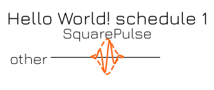
We start by defining a SquarePulse with a 5 GHz carrier and a duration of 100 ns. (For a full list of pre-defined pulse shapes see Operations)

[1]:

from qblox_scheduler import ClockResource, Schedule
from qblox_scheduler.operations import SquarePulse

schedule = Schedule(name="Hello World!")

# Add a clock used to generate the modulated output
schedule.add_resource(ClockResource(name="q0.01", freq=5.0e9))

# Add a pulse to the schedule
p1 = schedule.add(SquarePulse(amplitude=1, duration=100e-9, port="q0:mw", clock="q0.01"))

schedule.plot_circuit_diagram()

[1]:

(<Figure size 1000x100 with 1 Axes>,
 <Axes: title={'center': 'Hello World! schedule 1'}>)

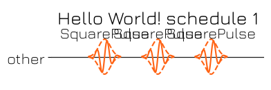
../../_images/quickstart_QBS_helloworld_qbloxscheduler_helloworld_1_1.png

We can add more pulses and set explicit timing between them. This is done with the help of the ref_op and rel_time keywords:

[2]:

# add the pulse rel_time=10ns referenced to the first square pulse p1
p2 = schedule.add(
    SquarePulse(amplitude=0.35, duration=70e-9, port="q0:mw", clock="q0.01"),
    rel_time=10e-9,
    ref_op=p1,
)

# add the pulse 150ns after the first pulse
p3 = schedule.add(
    SquarePulse(amplitude=0.65, duration=100e-9, port="q0:mw", clock="q0.01"),
    rel_time=150e-9,
    ref_op=p1,
)
schedule.plot_circuit_diagram()

[2]:

(<Figure size 1000x100 with 1 Axes>,
 <Axes: title={'center': 'Hello World! schedule 1'}>)

../../_images/quickstart_QBS_helloworld_qbloxscheduler_helloworld_3_1.png

Compiling Schedules and Hardware configuration#

In order to run the described above pulse sequence it needs to be first compiled into a set of low-level instructions for the Q1 processor. First, we need to define the target hardware for the schedule. The general structure is:

[3]:

from qblox_scheduler import HardwareAgent

hardware_cfg = {
    "config_type": "QbloxHardwareCompilationConfig",
    "hardware_description": {
        ### description of the cluster configuration: installed modules
    },
    "connectivity": {
        ### description of the links between the cluster physical inputs/outputs and the logical ports of the DUT
    },
    "hardware_options": {
        ### static device settings such as output attenuation, modulation frequencies etc.
    },
}

💡 Note: in practice the Hardware configuration is stored and passed as a JSON file

In this first example, we will configure a Qblox Cluster with a single Qubit Readout Module (QRM-RF) installed in slot 2.

The QRM-RF provides one output (O1) and one input (I1) operating in the 2–18.5 GHz range. To keep things simple, we will only configure the microwave output for now by mapping this physical channel to the DUT’s logical port, q0:mw (where q0 represents qubit 0, and mw represents the microwave drive).

In the final section of the hardware configuration (hardware_options) we can setup experimental parameters such as attenuation, Local Oscillator (LO) frequency, Intermediate Frequency (IF), and more.

To enable microwave modulation, we assign a local oscillator frequency to the DUT’s microwave input. This is done using the q0:mw-q0.01 key, which follows a strict {port}-{clock} naming convention:

q0:mw: The logical port defined in the connectivity graph
q0.01: A clock that tracks the operation frequency of the qubit (in this case, the transition |0> to |1> state)

We will dive deeper into the ports and clocks naming convention later in the notebook.

[4]:

# Describe the used Qblox cluster and installed modules
hardware_cfg["hardware_description"] = {
    "cluster0": {  # cluster name
        "instrument_type": "Cluster",
        "modules": {"2": {"instrument_type": "QRM_RF"}},  # Dictionary of installed modules
        "ip": None,  # e.g. "192.168.0.2" or None to use with a dummy cluster,
        "ref": "internal",  # reference clock internal/external
    }
}

# Declare the device inputs and outputs
hardware_cfg["connectivity"] = {
    "graph": [
        ("cluster0.module2.complex_output_0", "q0:mw"),  # (physical port, DUT_Name:DUT_Port)
        ("cluster0.module2.complex_input_0", "q0i:ro"),
    ]
}

hardware_cfg["hardware_options"] = {"modulation_frequencies": {"q0:mw-q0.01": {"lo_freq": 5.0e9}}}

Now we have defined our hardware configuration and we want to execute a Qblox Scheduler program on the hardware. To do so, we introduce an object called HardwareAgent to facilitate the communication with our hardware.

Hardware Agent#

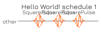
The HardwareAgent is a Qblox Scheduler Object, which transmits the created schedules in Qblox Scheduler to the Qblox Cluster. The HardwareAgent takes the created schedule as input, compiles it to Q1ASM and executes it on the hardware. To let the HardwareAgent know what hardware it will communicate to, we have to pass the name of our hardware configuration file as an argument:

[5]:

agent = HardwareAgent(hardware_cfg)
schedule.plot_circuit_diagram()
sched = agent.compile(schedule)

/.venv/lib/python3.14/site-packages/qblox_scheduler/qblox/hardware_agent.py:572: UserWarning: cluster0: Trying to instantiate cluster with ip 'None'.Creating a dummy cluster.
  warnings.warn(

../../_images/quickstart_QBS_helloworld_qbloxscheduler_helloworld_9_1.png

We can visualize the compiled pulse sequence:

[6]:

sched.plot_pulse_diagram(plot_backend="plotly")

Gate-level Description and DUT Configuration#

Furthermore, the qblox-scheduler enables a gate-level description of a quantum-circuit. Let’s add an Rxy(theta, phi)rotation to the schedule:

[7]:

from qblox_scheduler.operations import Rxy

# Add an Rxy gate 10ns after the last square pusle
schedule.add(Rxy(theta=35, phi=0, qubit="q0"), ref_op=p3, rel_time=10e-9)
schedule.plot_circuit_diagram()

[7]:

(<Figure size 1000x100 with 1 Axes>,
 <Axes: title={'center': 'Hello World! schedule 1'}>)

findfont: Failed to find font weight 300, now using 400.
findfont: Failed to find font weight 300, now using 400.
findfont: Failed to find font weight 300, now using 400.
findfont: Failed to find font weight 300, now using 400.
findfont: Failed to find font weight 300, now using 400.
findfont: Failed to find font weight 300, now using 400.
findfont: Failed to find font weight 300, now using 400.
findfont: Failed to find font weight 300, now using 400.
findfont: Failed to find font weight 300, now using 400.
findfont: Failed to find font weight 300, now using 400.
findfont: Failed to find font weight 300, now using 400.
findfont: Failed to find font weight 300, now using 400.
findfont: Failed to find font weight 300, now using 400.
findfont: Failed to find font weight 300, now using 400.
findfont: Failed to find font weight 300, now using 400.
findfont: Failed to find font weight 300, now using 400.
findfont: Failed to find font weight 300, now using 400.
findfont: Failed to find font weight 300, now using 400.
findfont: Failed to find font weight 300, now using 400.
findfont: Failed to find font weight 300, now using 400.
findfont: Failed to find font weight 300, now using 400.

../../_images/quickstart_QBS_helloworld_qbloxscheduler_helloworld_14_2.png

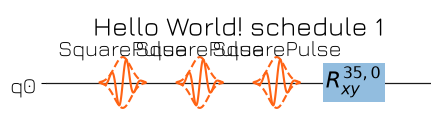
This gate-level description is entirely independent of the underlying qubit hardware implementation.

To make our gate-level descriptions meaningful, the compiler needs a physical model of our qubit. In qblox-scheduler, this is handled by a DeviceElement. For this example, we will assume our device under test is a fixed-frequency trasnmon qubit modeled by the BasicTransmonElement.

💡 Learn More: You can check out the Device Elements Documentation for a list of existing device classes, or follow the Custom Device Elements Tutorial to learn how to define your own.

[8]:

from qblox_scheduler import BasicTransmonElement, QuantumDevice

# Create the top-level device under test (DUT)
dut = QuantumDevice("DUT")

# Create the transmon element and add it to the device
qubit = BasicTransmonElement(name="q0")
dut.add_element(qubit)

# Explore the qubit ports and clocks:
print("Transmon Ports:", qubit.ports)
print("Transmon Clocks:", qubit.clock_freqs)

# Set the Rxy pulse amplitude
qubit.rxy.amp180 = 0.65

Transmon Ports: name='ports' microwave='q0:mw' flux='q0:fl' readout='q0:res'
Transmon Clocks: name='clock_freqs' f01=nan f12=nan readout=nan

/tmp/ipykernel_10358/3699729381.py:1: FutureWarning:

'BasicTransmonElement' will be removed in 1.0 and made available in a separate repository, see release notes for more details.

Notice how the printed ports match the “q0:mw” identifier we used earlier in our hardware configuration.

As for the frequencies, the element tracks three distinct clock channels.

q0.01 = f01: The fundamental qubit frequency (the \(\vert 0 \rangle \rightarrow \vert 1 \rangle\) transition)
q0.12 = f12: The next higher excited state frequency (the \(\vert 1 \rangle \rightarrow \vert 2 \rangle\) transition)
q0.ro = readout: The resonator frequency used for readout

💡 Note: in practice the DUT configuration is stored and passed as a JSON file

With the definitions over, we can compile and run the schedule:

[9]:

agent = HardwareAgent(hardware_cfg, dut)
data = agent.run(schedule=schedule)

# display the acquired data (we are not measuring, so it will return empty)
print(data)

# and the final pulse sequence
agent.latest_compiled_schedule.plot_pulse_diagram(plot_backend="plotly")

/.venv/lib/python3.14/site-packages/qblox_scheduler/qblox/hardware_agent.py:572: UserWarning:

cluster0: Trying to instantiate cluster with ip 'None'.Creating a dummy cluster.

<xarray.Dataset> Size: 0B
Dimensions:  ()
Data variables:
    *empty*
Attributes:
    tuid:     20260903-205357-662-763f21