Measuring \(g^2\)-correlation using QTM#

Second-order photon correlation measurements \((g^2)\) are fundamental in quantum optics. Amongst many other applications, it can provide a clear signature of single-photon emission and enables the validation of quantum light sources. Color centers are for instance a typical example of such single photon emitter.

The second-order correlation function \(g^2(\tau)\) can be computed out of a single detection mode – one would generally call it local correlations or autocorrelation – or between two detection modes – in that case one would typically call it crossed or sometimes non-local correlations. The latter case is for instance considered in the Hanbury Brown and Twiss (HBT) interferometry experiment. We invite the interested reader to refer to the following references for a more in-depth discussion of the HBT effect and correlation measurements:

Brown, R.H., Twiss, R.Q., 1956. Correlation between Photons in two Coherent Beams of Light. Nature 177, 27–29.
Grangier, P., Roger, G., Aspect, A., 1986. Experimental Evidence for a Photon Anticorrelation Effect on a Beam Splitter: A New Light on Single-Photon Interferences. Europhys. Lett. 1, 173–179.
Mandel, L., Wolf, E., 1995. Optical Coherence and Quantum Optics, 1st ed. Cambridge University Press.
Gerry, C., Knight, P., 2004. Introductory Quantum Optics, 1st ed. Cambridge University Press.

Correlation functions (of any order) are characteristic of the light source\({}^\dagger\) and provides valuable experimental information about it. For example, in photonics, a dip below \(0.5\) of the autocorrelation function at zero time delay indicates that single photons are detected. In the context of color centers, this allows to subsequently conclude that these photons originate from a single color center\({}^\ddagger\).

\({}^\dagger\): also applicable to other types of interferometric resources, such as electrons or atoms. \({}^\ddagger\): Shuo Li, Wenchao Li, Vladislav V. Yakovlev, Allison Kealy, and Andrew D. Greentree, “En route to nanoscopic quantum optical imaging: counting emitters with photon-number-resolving detectors,” Opt. Express 30, 12495-12509 (2022)

Description of the example experiment#

In this demo, we use the Qubit Timetag Module (QTM) to perform a \(g^2\) measurement. Two input channels of the QTM are used to record the detection events, enabling correlation analysis. A simplified schematic of a possible corresponding setup is shown below:

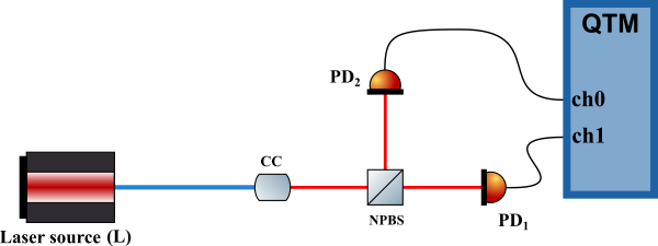
d238b239a7d74152bc7c8ae4d904e3b2

A coherent laser beam (in red) is exciting a single photon emitter, for instance a color center in diamond (CC). The emitted photons (following the blue path) are then split by a beam splitter (BS) and detected by two single photon detectors (PD) and timetagged by the QTM. A single photon cannot be detected by both detectors detectors monitoring each output port of the beam splitter, consequently, the crossed correlation function \(g^2(\tau)\) between both channels is expected to be \(0\) at \(\tau=0\).

[1]:

import numpy as np
from data_analysis import G2Correlation

from quantify_core.data import handling as dh
from quantify_scheduler import QuantumDevice, Schedule, SerialCompiler
from quantify_scheduler.enums import BinMode, TimeRef
from quantify_scheduler.operations import TimetagTrace

from utils import initialize_hardware, run_schedule

Setting up the hardware for the measurement#

!qblox-pnp list

[2]:

# Setup quantify output directory
dh.set_datadir(dh.default_datadir())
# Load and define the Hardware configuration
device_path = "devices/nv_center1q.json"
config_path = "configs/nv_center_qrm.json"

Data will be saved in:
/root/quantify-data

Quantum device settings#

[3]:

quantum_device = QuantumDevice.from_json_file(device_path)
quantum_device.hardware_config.load_from_json_file(config_path)

qubit = quantum_device.get_element("qe0")

[4]:

cluster_ip = None  # Fill in the ip to run this tutorial on hardware,
measctrl, ic, cluster = initialize_hardware(quantum_device, cluster_ip)
compiler = SerialCompiler(name="compiler")

Schedule for \(g^{(2)}\)-correlation using `TimetagTrace` acquisition#

To time-stamp the incoming photons on any channel of QTM, we use TimetagTrace acquisition in Quantify, where it can record a stream of timetags within a defined acquisition window (duration) defined as how long photon arrivals are acquired. Every time there is a rising edge detected, a timetag is recorded.

Here, we add the TimetagTrace in channel 0 and channel 1, with each acquisition window of \(50~\mu s\).

[5]:

ACQUISITION_TIME = 50e-6  # 50 us

main_schedule = Schedule("g2_schedule")

# Adding TimetagTrace on channel 0
main_schedule.add(
    TimetagTrace(
        duration=ACQUISITION_TIME,
        port="qtm0:in",
        clock="digital",
        acq_channel=0,
        bin_mode=BinMode.APPEND,
        time_ref=TimeRef.START,
    ),
    ref_pt="start",
)

# Adding TimetagTrace on channel 1
main_schedule.add(
    TimetagTrace(
        duration=ACQUISITION_TIME,
        port="qtm1:in",
        clock="digital",
        acq_channel=1,
        bin_mode=BinMode.APPEND,
        time_ref=TimeRef.START,
    ),
    ref_pt="start",
    rel_time=0,
)

[5]:

{'name': '3dc1ac96-e709-4bc0-a016-25b535b464ac', 'operation_id': '1664845176180229549', 'timing_constraints': [{'rel_time': 0, 'ref_schedulable': None, 'ref_pt_new': None, 'ref_pt': 'start'}], 'label': '3dc1ac96-e709-4bc0-a016-25b535b464ac'}

We compile the schedule.

[6]:

compiled_schedule = compiler.compile(
    schedule=main_schedule,
    config=quantum_device.generate_compilation_config(),
)

And we execute it on the hardware. To illustrate the behavior of a single color center, we present a set of simulated time-tags that replicate the expected \(g^{(2)}\) correlation signature.

[7]:

if cluster_ip is not None:  # if running on hardware
    acquisition = run_schedule(compiled_schedule, quantum_device)
    time_tags1 = acquisition.isel()[0].values[0][0]
    time_tags2 = acquisition.isel()[1].values[0][0]
else:
    # in case of dummy cluster, we use the simulated time tags for single photon emission
    time_tags1, time_tags2 = np.load("simulated_timetags.npz").values()

Measuring \(g^{(2)} (\tau)\)#

[8]:

# Calculate g2 for the obtained time-tags
g2_corr_experiment = G2Correlation(time_tags1, time_tags2, 10)
g2_corr_experiment.plot_data("Experiment", plot_fit=True)

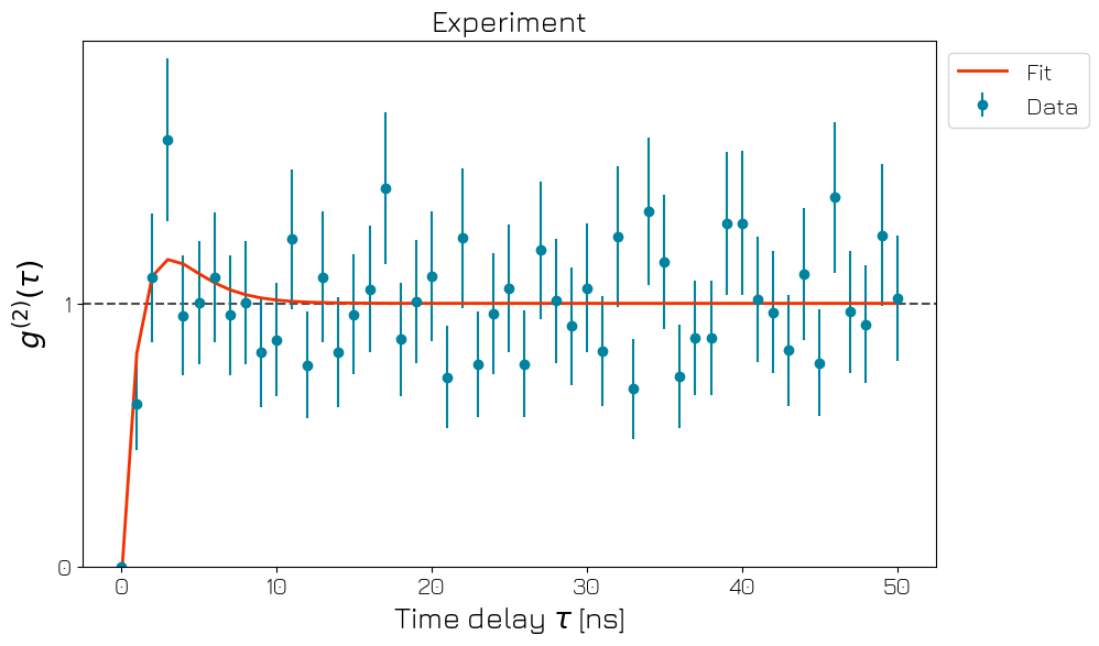
../../../_images/applications_quantify_nv_center_g2_16_0.png

In the example above we exhibit the second-order cross correlations between two simulated photo-detection events, as might be observed at the output of a beam splitter fed by a single-photon source (e.g., a color center in diamond). This experiment has been first described and performed in the following reference: Grangier, P., Roger, G., Aspect, A., 1986.. Therefore, in the observed plot above, \(g^{(2)}(\tau=0)=0\), verifying the presence of a single quantum emitter.

Of course, the technical implementation of Quantify and Qblox hardware shown in this application example is also suitable for any other kind of experiment involving the measurement of the second-order correlation function, out of two separated detection channels. For instance, the Hanbury Brown and Twiss experiment is another famous example of such setup.