See also
A Jupyter notebook version of this tutorial can be downloaded here.

Coupled qubits characterization#
The experiments of this tutorial are meant to be executed with a Qblox Cluster controlling a flux-tunable transmon system.
The experiments can also be executed using a dummy Qblox device that is created via an instance of the Cluster class, and is initialized with a dummy configuration. However, when using a dummy device, the analysis will not work because the experiments will return np.nan values.
Hardware setup#
In this section we configure the hardware configuration which specifies the connectivity of our system.
Configuration file#
This is a template hardware configuration file for a 2-qubit system (we name the qubits q0 and q1), with dedicated flux-control lines.
The hardware setup is as follows, by cluster slot:
QCM-RF (Slot 6)
Drive line for
q0using fixed 80 MHz IF.Drive line for
q1using fixed 80 MHz IF.
QCM (Slot 2)
Flux line for
q0.Flux line for
q1.
QRM-RF (Slot 8)
Shared readout line for
q0/q1using a fixed LO set at 7.5 GHz.
Note that in the hardware configuration below the mixers are uncorrected, but for high fidelity experiments this should also be done for all the modules.
[1]:
import json

import rich
[2]:
with open("configs/tuning_transmon_coupled_pair_hardware_config.json") as hw_cfg_json_file:
    hardware_cfg = json.load(hw_cfg_json_file)
Scan For Clusters#
We scan for the available devices connected via ethernet using the Plug & Play functionality of the Qblox Instruments package (see Plug & Play for more info).
!qblox-pnp list
[3]:
cluster_ip = None  # To run this tutorial on hardware, fill in the IP address of the cluster here
cluster_name = "cluster0"
Connect to Cluster#
We now make a connection with the Cluster.
[4]:
from qcodes.instrument import find_or_create_instrument

from qblox_instruments import Cluster, ClusterType

cluster = find_or_create_instrument(
    Cluster,
    recreate=True,
    name=cluster_name,
    identifier=cluster_ip,
    dummy_cfg=(
        {
            2: ClusterType.CLUSTER_QCM,
            4: ClusterType.CLUSTER_QRM,
            6: ClusterType.CLUSTER_QCM_RF,
            8: ClusterType.CLUSTER_QRM_RF,
        }
        if cluster_ip is None
        else None
    ),
)
Experiment setup#
Quantum device settings#
Here we initialize our QuantumDevice and our qubit parameters, checkout this tutorial for further details.
In short, a QuantumDevice contains device elements where we save our found parameters.
This tutorial explicitly only deals with 2-qubit experiments. As such, we assume that both the qubits and their resonators have already been characterized. For information on how to do this, please see the single transmon qubit tutorial.
[5]:
from quantify_scheduler.device_under_test.quantum_device import QuantumDevice

quantum_device = QuantumDevice.from_json_file("devices/transmon_device_2q.json")
q0 = quantum_device.get_element("q0")
q1 = quantum_device.get_element("q1")
quantum_device.hardware_config(hardware_cfg)
Configure measurement control loop#
We will use a MeasurementControl object for data acquisition as well as an InstrumentCoordinator for controlling the instruments in our setup.
The PlotMonitor is used for live plotting.
All of these are then associated with the QuantumDevice.
[6]:
from quantify_core.measurement.control import MeasurementControl
from quantify_core.visualization.pyqt_plotmon import PlotMonitor_pyqt as PlotMonitor
from quantify_scheduler.instrument_coordinator import InstrumentCoordinator
from quantify_scheduler.instrument_coordinator.components.qblox import ClusterComponent


def configure_measurement_control_loop(
    device: QuantumDevice, cluster: Cluster, live_plotting: bool = False
):
    meas_ctrl = find_or_create_instrument(MeasurementControl, recreate=True, name="meas_ctrl")
    ic = find_or_create_instrument(InstrumentCoordinator, recreate=True, name="ic")

    # Add cluster to instrument coordinator
    ic_cluster = ClusterComponent(cluster)
    ic.add_component(ic_cluster)

    if live_plotting:
        # Associate plot monitor with measurement controller
        plotmon = find_or_create_instrument(PlotMonitor, recreate=False, name="PlotMonitor")
        meas_ctrl.instr_plotmon(plotmon.name)

    # Associate measurement controller and instrument coordinator with the quantum device
    device.instr_measurement_control(meas_ctrl.name)
    device.instr_instrument_coordinator(ic.name)

    return (meas_ctrl, ic)


meas_ctrl, instrument_coordinator = configure_measurement_control_loop(quantum_device, cluster)
Set data directory#
This directory is where all of the experimental data as well as all of the post processing will go.
[7]:
import quantify_core.data.handling as dh

# Enter your own dataset directory here!
dh.set_datadir(dh.default_datadir())
Data will be saved in:
/root/quantify-data
Configure external flux control#
We need to have some way of controlling the external flux.
This can be done by setting an output bias on a module of the cluster which is then connected to the flux-control line.
Here we are nullifying the external flux on both qubits.
[8]:
flux_settables = {q0.name: cluster.module2.out0_offset, q1.name: cluster.module2.out1_offset}

for flux_settable in flux_settables.values():
    flux_settable.inter_delay = 100e-9  # Delay time in seconds between consecutive set operations.
    flux_settable.step = 0.3e-3  # Stepsize in V that this Parameter uses during set operation.
    flux_settable()  # Get before setting to avoid jumps.
    flux_settable(0.0)
[9]:
flux_settables[q0.name](0.0)  # enter your own value here for qubit 0
flux_settables[q1.name](0.0)  # enter your own value here for qubit 1
Activate NCO delay compensation#
Compensate for the digital propagation delay for each qubit (i.e each sequencer)
For more info, please see: https://docs.qblox.com/en/main/api_reference/sequencer.html#Sequencer.nco_prop_delay_comp
To avoid mismatches between modulation and demodulation, the delay between any readout frequency or phase changes and the next acquisition should be equal or greater than the total propagation delay (146ns + user defined value).
[10]:
for i in range(6):
    getattr(cluster.module8, f"sequencer{i}").nco_prop_delay_comp_en(True)
    getattr(cluster.module8, f"sequencer{i}").nco_prop_delay_comp(10)
Experiments#
As in the single qubit tuneup tutorial, the sweep setpoints for all experiments in this section are only examples. The sweep setpoints should be changed to match your own system. In this section we assume that each individual qubit has already been characterized, and that they have been biased to their sweetspots.
We will examine the flux response of the 2-qubit system. By “flux response” we mean the measured response of the system when the parameterization of a flux pulse is varied.
We consider two separate experiments which have their own separate parameterizations, they are:
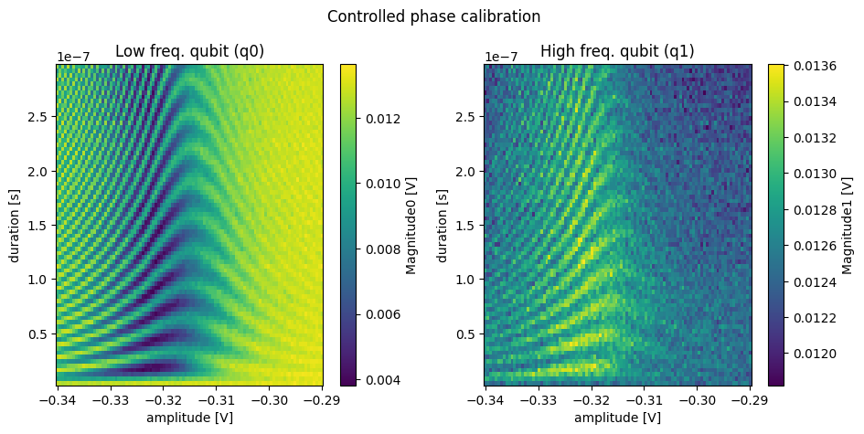
Controlled phase calibration (a.k.a. two-qubit Chevron experiment)
Used to measure coupling strength between the two qubits.
Used to find the location of the \(|11\rangle \leftrightarrow |02\rangle\) avoided crossing.
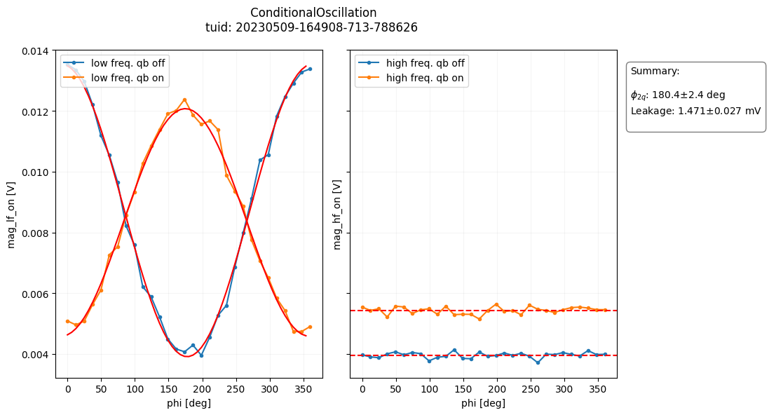
Conditional oscillations
Used to measure the conditional phase of the controlled phase gate.
Used to estimate leakage to \(|02\rangle\).
Can also be used to measure single-qubit phases on the individual qubits.
In both of these experiments, we apply the flux pulse on the flux-control line of q1 (on top of the sweetspot bias) which we take to be the qubit with the higher frequency, i.e. \(\omega_1\) > \(\omega_0\).
Controlled phase calibration#
[11]:
import numpy as np
from qcodes.parameters import ManualParameter

from quantify_scheduler import Schedule
from quantify_scheduler.gettables import ScheduleGettable
from quantify_scheduler.operations.gate_library import Measure, Reset, X
from quantify_scheduler.schedules.two_qubit_transmon_schedules import chevron_cz_sched
[12]:
duration = ManualParameter(name="dur", unit="Hz", label="Duration of flux pulse")
amplitude = ManualParameter(name="amp", unit="", label="Amplitude of flux pulse")

amplitude.batched = True
duration.batched = False

chevron_cz_sched_kwargs = dict(
    lf_qubit=q0.name, hf_qubit=q1.name, amplitudes=amplitude, duration=duration
)

gettable = ScheduleGettable(
    quantum_device,
    schedule_function=chevron_cz_sched,
    schedule_kwargs=chevron_cz_sched_kwargs,
    real_imag=False,
    data_labels=[
        "Magnitude lf qubit",
        "Phase lf qubit",
        "Magnitude hf qubit",
        "Phase hf qubit",
    ],
    batched=True,
    num_channels=2,
)

meas_ctrl.gettables(gettable)
[13]:
quantum_device.cfg_sched_repetitions(400)

duration_setpoints = np.arange(4e-9, 20e-9, 4e-9)
amplitude_setpoints = np.linspace(0.05, 0.2, 10)

meas_ctrl.settables([duration, amplitude])
meas_ctrl.setpoints_grid((duration_setpoints, amplitude_setpoints))

chevron_ds = meas_ctrl.run("chevron")
chevron_ds
Starting batched measurement...
Iterative settable(s) [outer loop(s)]:
         dur
Batched settable(s):
         amp
Batch size limit: 40
[13]:
<xarray.Dataset> Size: 2kB
Dimensions:  (dim_0: 40)
Coordinates:
    x0       (dim_0) float64 320B 4e-09 4e-09 4e-09 ... 1.6e-08 1.6e-08 1.6e-08
    x1       (dim_0) float64 320B 0.05 0.06667 0.08333 0.1 ... 0.1667 0.1833 0.2
Dimensions without coordinates: dim_0
Data variables:
    y0       (dim_0) float64 320B nan nan nan nan nan ... nan nan nan nan nan
    y1       (dim_0) float64 320B nan nan nan nan nan ... nan nan nan nan nan
    y2       (dim_0) float64 320B nan nan nan nan nan ... nan nan nan nan nan
    y3       (dim_0) float64 320B nan nan nan nan nan ... nan nan nan nan nan
Attributes:
    tuid:                             20250811-125444-760-b6b6c4
    name:                             chevron
    grid_2d:                          True
    grid_2d_uniformly_spaced:         True
    1d_2_settables_uniformly_spaced:  False
    xlen:                             4
ylen: 10Conditional oscillations#
[14]:
from typing import Literal

from numpy.typing import NDArray

from quantify_scheduler.operations import X90, Rxy, SuddenNetZeroPulse


def conditional_oscillation_sched(
    target_qubit: str,
    control_qubit: str,
    phases: NDArray,
    variant: Literal["OFF", "ON"],
    snz_A: float,
    snz_B: float,
    snz_scale: float,
    snz_dur: float,
    snz_t_phi: float,
    snz_t_integral_correction: float,
    flux_port: str = None,
    repetitions: int = 1,
) -> Schedule:
    """
    Make a conditional oscillation schedule to measure conditional phase.

    Parameters
    ----------
    target_qubit
        The name of a qubit, e.g., "q0", the qubit with lower frequency.
    control_qubit
        The name of coupled qubit, the qubit with the higher frequency.
    phases
        An array (or scalar) of recovery phases in degrees.
    variant
        A string specifying whether to excite the control qubit.
    snz_A
        Unitless amplitude of the main square pulse.
    snz_B
        Unitless scaling correction for the final sample of the first
        square and first sample of the second square pulse.
    snz_scale
        Amplitude scaling correction factor of the negative arm of the net-zero pulse.
    snz_dur
        The total duration of the two half square pulses.
    snz_t_phi
        The idling duration between the two half pulses.
    snz_t_integral_correction
        The duration in which any non-zero pulse amplitude needs to be corrected.
    flux_port
        An optional string for a flux port. Default is hf_qubit flux port.
    repetitions
        The amount of times the Schedule will be repeated.

    Returns
    -------
    :
        An experiment schedule.

    """
    sched = Schedule(f"ConditionalOscillation({variant})", repetitions)

    # Ensure phases is an iterable when passing a float
    phases = np.asarray(phases)
    phases = phases.reshape(phases.shape or (1,))

    # Ensure that variant is uppercase for switch
    variant = str.upper(variant)
    if variant not in {"OFF", "ON"}:
        raise ValueError("Schedule variant should be 'OFF' or 'ON'.")

    # Set flux port
    flux_port = flux_port if flux_port is not None else f"{control_qubit}:fl"

    for acq_index, phi in enumerate(phases):
        # Reset to |00>
        sched.add(Reset(target_qubit, control_qubit))

        # Apply a pi/2 pulse on the target qubit
        targ_eq_ref = sched.add(X90(target_qubit))

        if variant == "ON":
            # Also apply a pi pulse on the control qubit
            sched.add(X(control_qubit), ref_op=targ_eq_ref, ref_pt="start")

        # Go to |11> <=> |02> avoided crossing on positive & negative sides
        # using the SuddenNetZeroPulse
        sched.add(
            SuddenNetZeroPulse(
                amp_A=snz_A,
                amp_B=snz_B,
                net_zero_A_scale=snz_scale,
                t_pulse=snz_dur,
                t_phi=snz_t_phi,
                t_integral_correction=snz_t_integral_correction,
                port=flux_port,
                clock="cl0.baseband",
            )
        )

        # Apply a pi/2 recovery pulse on the target qubit
        targ_rec_ref = sched.add(Rxy(theta=90.0, phi=phi, qubit=target_qubit))

        if variant == "ON":
            # Also apply a pi pulse on the control qubit
            sched.add(X(control_qubit), ref_op=targ_rec_ref, ref_pt="start")

        # Measure system
        sched.add(Measure(target_qubit, control_qubit, acq_index=acq_index))

    return sched
[15]:
phase = ManualParameter(name="ph", unit="deg", label="Recovery phase")
flux_pulse_amplitude = ManualParameter(name="A", unit="", label="Flux pulse amplitude")
scaling_correction = ManualParameter(name="B", unit="", label="Scaling correction")

phase.batched = True
flux_pulse_amplitude.batched = False
scaling_correction.batched = False

conditional_oscillation_sched_kwargs = dict(
    target_qubit=q0.name,
    control_qubit=q1.name,
    phases=phase,
    snz_A=flux_pulse_amplitude,
    snz_B=scaling_correction,
    snz_scale=1.0,
    snz_dur=40e-9,
    snz_t_phi=4e-9,
    snz_t_integral_correction=0.0,
)

gettable_off = ScheduleGettable(
    quantum_device,
    conditional_oscillation_sched,
    schedule_kwargs={**conditional_oscillation_sched_kwargs, **{"variant": "OFF"}},
    real_imag=False,
    batched=True,
    num_channels=2,
)
gettable_on = ScheduleGettable(
    quantum_device,
    conditional_oscillation_sched,
    schedule_kwargs={**conditional_oscillation_sched_kwargs, **{"variant": "ON"}},
    real_imag=False,
    batched=True,
    num_channels=2,
)

meas_ctrl.gettables((gettable_off, gettable_on))
[16]:
quantum_device.cfg_sched_repetitions(400)

meas_ctrl.settables([phase, flux_pulse_amplitude, scaling_correction])
meas_ctrl.setpoints_grid((np.linspace(0.0, 360.0, 60), [0.8], [0.5]))

cond_osc_ds = meas_ctrl.run("conditional oscillation")
cond_osc_ds
Starting batched measurement...
Iterative settable(s) [outer loop(s)]:
         A, B
Batched settable(s):
         ph
Batch size limit: 60
/builds/0/.venv/lib/python3.9/site-packages/quantify_scheduler/waveforms.py:364: RuntimeWarning: divide by zero encountered in scalar divide
  integral_value = -sum(waveform) / num_corr_samples
/builds/0/.venv/lib/python3.9/site-packages/quantify_scheduler/waveforms.py:364: RuntimeWarning: divide by zero encountered in scalar divide
  integral_value = -sum(waveform) / num_corr_samples
[16]:
<xarray.Dataset> Size: 5kB
Dimensions:  (dim_0: 60)
Coordinates:
    x0       (dim_0) float64 480B 0.0 6.102 12.2 18.31 ... 347.8 353.9 360.0
    x1       (dim_0) float64 480B 0.8 0.8 0.8 0.8 0.8 ... 0.8 0.8 0.8 0.8 0.8
    x2       (dim_0) float64 480B 0.5 0.5 0.5 0.5 0.5 ... 0.5 0.5 0.5 0.5 0.5
Dimensions without coordinates: dim_0
Data variables:
    y0       (dim_0) float64 480B nan nan nan nan nan ... nan nan nan nan nan
    y1       (dim_0) float64 480B nan nan nan nan nan ... nan nan nan nan nan
    y2       (dim_0) float64 480B nan nan nan nan nan ... nan nan nan nan nan
    y3       (dim_0) float64 480B nan nan nan nan nan ... nan nan nan nan nan
    y4       (dim_0) float64 480B nan nan nan nan nan ... nan nan nan nan nan
    y5       (dim_0) float64 480B nan nan nan nan nan ... nan nan nan nan nan
    y6       (dim_0) float64 480B nan nan nan nan nan ... nan nan nan nan nan
    y7       (dim_0) float64 480B nan nan nan nan nan ... nan nan nan nan nan
Attributes:
    tuid:                             20250811-125445-938-0fff8a
    name:                             conditional oscillation
    grid_2d:                          False
    grid_2d_uniformly_spaced:         False
1d_2_settables_uniformly_spaced: False[17]:
rich.print(quantum_device.hardware_config())
{
    'config_type': 'quantify_scheduler.backends.qblox_backend.QbloxHardwareCompilationConfig',
    'hardware_description': {
        'cluster0': {
            'instrument_type': 'Cluster',
            'modules': {
                '6': {'instrument_type': 'QCM_RF'},
                '2': {'instrument_type': 'QCM'},
                '8': {'instrument_type': 'QRM_RF'}
            },
            'sequence_to_file': False,
            'ref': 'internal'
        }
    },
    'hardware_options': {
        'output_att': {'q0:mw-q0.01': 10, 'q1:mw-q1.01': 10, 'q0:res-q0.ro': 60, 'q1:res-q1.ro': 60},
        'mixer_corrections': {
            'q0:mw-q0.01': {
                'auto_lo_cal': 'on_lo_interm_freq_change',
                'auto_sideband_cal': 'on_interm_freq_change'
            },
            'q1:mw-q1.01': {
                'auto_lo_cal': 'on_lo_interm_freq_change',
                'auto_sideband_cal': 'on_interm_freq_change'
            },
            'q0:res-q0.ro': {
                'auto_lo_cal': 'on_lo_interm_freq_change',
                'auto_sideband_cal': 'on_interm_freq_change'
            },
            'q1:res-q1.ro': {
                'auto_lo_cal': 'on_lo_interm_freq_change',
                'auto_sideband_cal': 'on_interm_freq_change'
            }
        },
        'modulation_frequencies': {
            'q0:mw-q0.01': {'interm_freq': 80000000.0},
            'q1:mw-q1.01': {'interm_freq': 80000000.0},
            'q0:res-q0.ro': {'lo_freq': 7500000000.0},
            'q1:res-q1.ro': {'lo_freq': 7500000000.0}
        }
    },
    'connectivity': {
        'graph': [
            ['cluster0.module6.complex_output_0', 'q0:mw'],
            ['cluster0.module6.complex_output_1', 'q1:mw'],
            ['cluster0.module2.real_output_0', 'q0:fl'],
            ['cluster0.module2.real_output_1', 'q1:fl'],
            ['cluster0.module8.complex_output_0', 'q0:res'],
            ['cluster0.module8.complex_output_0', 'q1:res']
        ]
    }
}

