See also

A Jupyter notebook version of this tutorial can be downloaded here.

Pulsed ODMR for Color Centers

Introducing Color Centers

One of the commonly known color centers is Nitrogen-Vacancy (NV) centers in diamond. They are unique quantum systems with applications in quantum computing, sensing, and communications. In this notebook, we are going to use the qblox hardware to tune-up NV center qubit.

To use a NV-center as a quantum device, it must first be tuned and characterized. The process depends on the specific color center and involves sequential experiments, where each step builds on the results of the previous one. The workflow for tuning a color center is illustrated in the accompanying figure.

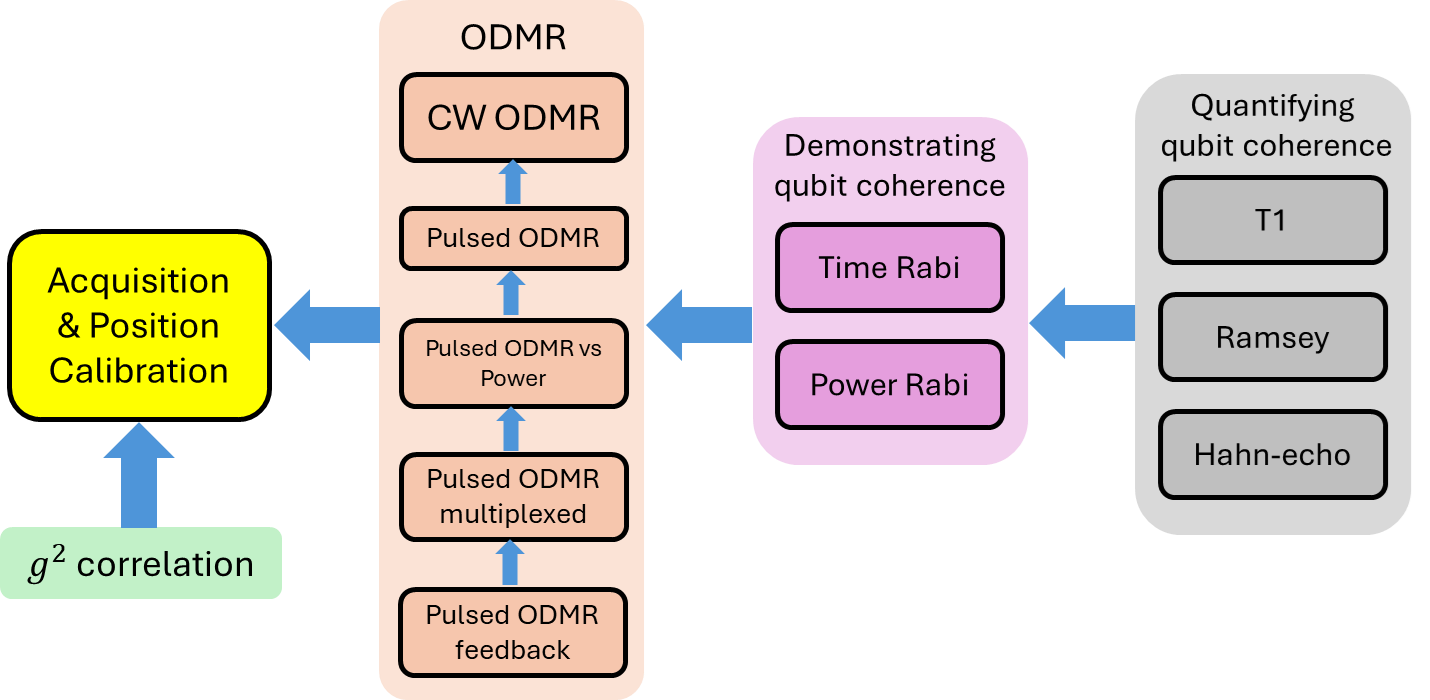
In this diagram, arrows indicate dependencies, showing that experiments are typically conducted from left to right.

One key experiment in characterizing color centers is Optically Detected Magnetic Resonance (ODMR), which is analogous to qubit spectroscopy. This notebook demonstrate two crucial methods, Pulsed ODMR and Pulsed ODMR with power, to measure the energy levels of an NV center.

from __future__ import annotations  # noqa: I001
import numpy as np
from nv_analysis import odmr_curve_fit
import pickle
from qcodes.instrument.parameter import ManualParameter
from quantify_core.data import handling as dh
from quantify_scheduler import QuantumDevice, Schedule, ScheduleGettable
from quantify_scheduler.enums import BinMode
from quantify_scheduler.operations import (
    Measure,
    SetClockFrequency,
    SquarePulse,
)
from quantify_scheduler.operations.shared_native_library import SpectroscopyOperation
from utils import initialize_hardware

Quantum device settings

Here we initialize our QuantumDevice and our qubit parameters, checkout this tutorial for further details.

In short, a QuantumDevice contains device elements where we save our found parameters. Here we are loading a template for 1 qubit.

device_path = "devices/nv_center1q.json"
config_path = "configs/nv_center_qrm.json"
dh.set_datadir(dh.default_datadir())

Data will be saved in:
/root/quantify-data

We define the QuantumDevice for NV center as nv_center. Next, we import the device and hardware config json file

nv_center = QuantumDevice.from_json_file(device_path)
qe0 = nv_center.get_element("qe0")
nv_center.hardware_config.load_from_json_file(config_path)
cluster_ip = None  # Fill in the ip to run this tutorial on hardware,

meas_ctrl, ic, cluster = initialize_hardware(
    nv_center, ip=cluster_ip
)  # to initialize the cluster and other instruments in hw config

Hardware Configuration Overview

Here, the NV center setup uses the Qubit Control Module (QCM) baseband module to control the acousto-optic modulator (AOM) for the readout laser. The QCM-RF II controls the qubit states \(|0\rangle\) and \(|1\rangle\) as the computational basis. Photon detectors (PD) are connected to the Qubit Readout Module (QRM) for counting fluorescent photons.

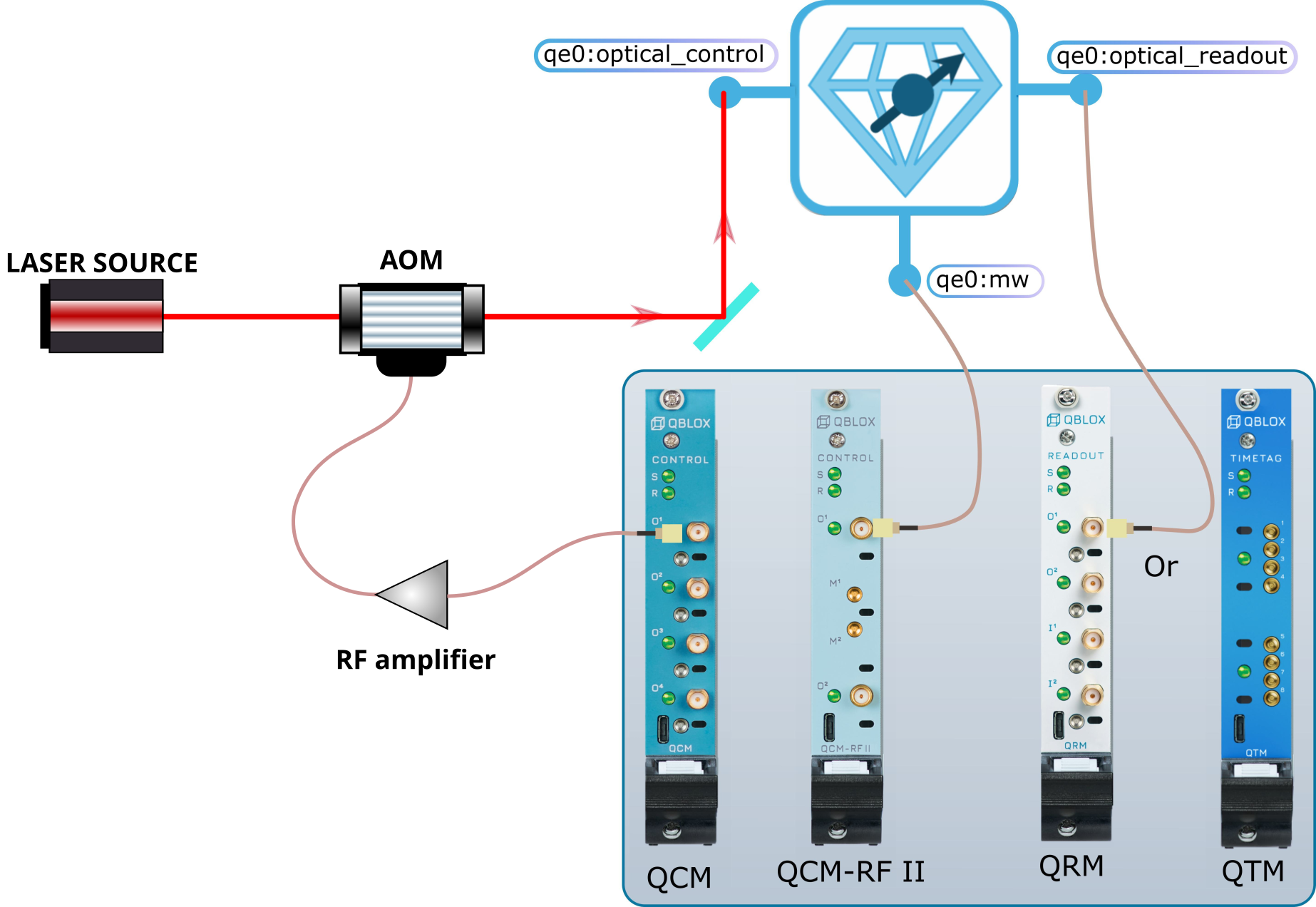
In the above figure, we show how a conventional NV center integrates qualitatively with the Qblox hardware. The hardware configuration (nv_center.hardware_config) translates this qualitative understanding into the specific backend setup required for the Qblox cluster.

• The readout laser is connected to the optical control port of the quantum device (qe0:optical_control). It is responsible for exciting the NV center to its fluorescent state.

• The acousto-optic modulator (AOM) precisely controls the readout laser, enabling modulation for optimal readout performance.

• To manipulate the \(|0\rangle\)-\(|1\rangle\) level, the microwave port of the qubit (qe0:mw) is connected to QCM-RF II.

• Finally, to measure photon counts, the optical readout port of the quantum device (qe0:optical_readout) is connected to QRM (or QTM).

More information about ports for NV center can be found here.

Pulsed ODMR Schedule

Pulsed Optically Detected Magnetic Resonance (ODMR) probes the \(|0\rangle\)-\(|1\rangle\) qubit transition by sweeping a microwave frequency using the QCM-RF II, which drives the transition when it matches the resonance frequency. The readout process involves activating the laser with the QCM to excite the color center, causing it to fluoresce, and detecting emitted photons with the QRM.

For NV centers:

• The \(|0\rangle\) state is the bright state, producing photon emissions when excited.

• The \(|1\rangle\) state is the dark state, resulting in negligible photon emissions.

The pulsed_odmr_freq consists for following steps:

1. Initialization

   • The readout laser is turned on for a fixed duration using a SquarePulse to initialize the qubit to \(|0\rangle\).

2. Microwave Frequency Sweep

   • The microwave frequency is set using SetClockFrequency at the qubit’s microwave port.

   • A SpectroscopyOperation applies the microwave tone, sweeping through frequencies to probe the \(|0\rangle\)-\(|1\rangle\) transition.

3. Readout

   • The Measure operation:

     • Activates the readout laser for a set duration, followed by acquisition with a time-of-flight delay.

     • Accumulates photon counts using bin_mode=BinMode.SUM, grouping results into a single bin per frequency across multiple repetitions.

def pulsed_odmr_freq(
    qubit: QuantumDevice,
    spec_frequencies: np.ndarray,
    repetitions: int = 1,
):
    """
    Construct a pulsed ODMR schedule.

    Args:
        qubit: The target qubit.
        spec_frequencies: Frequency or sweepable range of frequencies
        repetitions: Number of repetitions (default: 1).

    Returns:
        Schedule: A pulsed ODMR schedule.

    """
    # Initialize the schedule with the specified number of repetitions
    sched = Schedule("Pulsed ODMR", repetitions=repetitions)

    # Define control parameters

    clock_op = f"{qubit.name}.ge0"
    spec_clock = f"{qubit.name}.spec"

    port_op = f"{qubit.name}:optical_control"
    amp_op = qubit.measure.pulse_amplitude()
    duration_op = qubit.measure.pulse_duration()

    # Add an initial optical reset pulse
    sched.add(SquarePulse(amp=amp_op, duration=duration_op, port=port_op, clock=clock_op))

    # Add operations for each frequency
    for idx, spec_freq in enumerate(spec_frequencies):
        sched.add(SetClockFrequency(clock=spec_clock, clock_freq_new=spec_freq))
        sched.add(SpectroscopyOperation(qubit.name))  # MW pulse
        sched.add(Measure(qubit.name, acq_index=idx, bin_mode=BinMode.SUM))  # Measure

    return sched

Generate a range of frequencies with the defined steps for Pulsed ODMR spectroscopy

spec_freq_param = ManualParameter("spec_freq_param")
spec_freq_param.batched = True
frequency_steps = 10  # Set the number of frequency steps for the spectroscopy sweep
frequency_setpoints = np.linspace(2.52 * 1e9, 2.92 * 1e9, frequency_steps)

Setting the number of repetitions for the schedule

rep = 1
nv_center.cfg_sched_repetitions(rep)

Create a dictionary of parameters to pass to the pulsed ODMR function and initialize a ScheduleGettable to handle data acquisition with the schedule.

schedule_kwargs = {
    "qubit": qe0,  # Target qubit for ODMR
    "spec_frequencies": spec_freq_param,  # Frequencies for the sweep
}

Initialize the ScheduleGettable to handle data acquisition with the schedule.

pulsed_odmr_gettable = ScheduleGettable(
    quantum_device=nv_center,  # Quantum device object (NV center)
    schedule_function=pulsed_odmr_freq,  # Function defining the experiment sequence
    schedule_kwargs=schedule_kwargs,  # Parameters for the experiment schedule
    batched=True,  # Enable batched data acquisition
    data_labels=["Accumulative Counts"],  # Label for data output
)

Running the Experiment

meas_ctrl.settables([spec_freq_param])
meas_ctrl.setpoints_grid([frequency_setpoints])
meas_ctrl.gettables(pulsed_odmr_gettable)
dataset = meas_ctrl.run()

Starting batched measurement...
Iterative settable(s) [outer loop(s)]:
         --- (None) ---
Batched settable(s):
         spec_freq_param
Batch size limit: 10

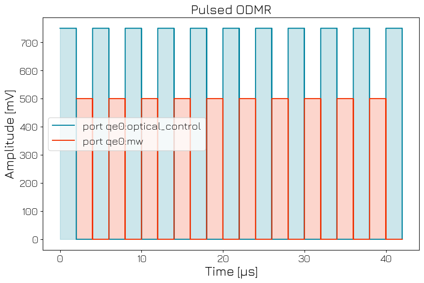
Looking at the Pulse Schedule Diagram

pulsed_odmr_gettable.compiled_schedule.plot_pulse_diagram()

(<Figure size 1000x621 with 1 Axes>,
 <Axes: title={'center': 'Pulsed ODMR'}, xlabel='Time [μs]', ylabel='Amplitude [mV]'>)

Analysis

Once measured the pulsed ODMR, the acquired data can be fitted to find the qubit transition frequency.

Here we analyse the experiment data taken for NV center at Fraunhofer IAF, Freiburg Germany with our modules.

# If using a dummy cluster, load the dataset from the example data
if cluster_ip is None:
    with open("pulsedodmr_one_amp_.pkl", "rb") as file:
        dataset = pickle.load(file)

transition_freq = odmr_curve_fit(dataset)

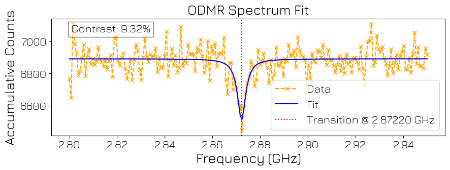
Transition Frequency: 2.87220 GHz with Contrast: 9.32%

Pulsed ODMR versus Power Schedule

To resolve the hyperfine structure of the qubit energy levels, pulsed ODMR is often performed across varying power levels. Additionally, after identifying the qubit’s transition frequency, optimizing the microwave power is crucial for better precision.

In Quantify, it’s easy to combine frequency and power sweeps within a single schedule. It only requires to add a few modifications to the existing pulsed_odmr_freq schedule.

In the newly defined pulsed_odmr schedule, the amplitudes to sweep over are provided via the spec_amps parameter. In the loop, for each frequency, the amplitude of the spectroscopy operation is adjusted, enabling efficient frequency and power optimization in one seamless schedule. It’s that simple!

def pulsed_odmr(
    qubit: QuantumDevice,
    spec_frequencies: np.ndarray,
    spec_amps: np.ndarray,
    repetitions: int = 1,
):
    """
    Construct a pulsed ODMR schedule.

    Args:
        qubit: Name of the target qubit.
        spec_frequencies: Frequency or sweepable range of frequencies.
        spec_amps: Amplitude or sweepable range of amplitudes.
        repetitions: Number of repetitions (default: 1).

    Returns:
        Schedule: A pulsed ODMR schedule.

    """
    # Initialize the schedule with the specified number of repetitions
    sched = Schedule("Pulsed ODMR", repetitions=repetitions)

    # Define control parameters
    port_op = f"{qubit.name}:optical_control"
    clock_op = f"{qubit.name}.ge0"
    spec_clock = f"{qubit.name}.spec"
    amp_op = qubit.measure.pulse_amplitude()
    duration_op = qubit.measure.pulse_duration()
    # Add an initial optical reset pulse
    sched.add(SquarePulse(amp=amp_op, duration=duration_op, port=port_op, clock=clock_op))

    # Add operations for each frequency and amplitude
    for idx, (spec_freq, spec_amp) in enumerate(zip(spec_frequencies, spec_amps)):
        sched.add(SetClockFrequency(clock=spec_clock, clock_freq_new=spec_freq))
        sched.add(SpectroscopyOperation(qubit.name, amplitude=spec_amp))  # MW pulse
        sched.add(Measure(qubit.name, acq_index=idx, bin_mode=BinMode.SUM))  # Measure

    return sched

In addition with defining the frequency setpoints, we define the amplitude setpoints as well.

spec_freq_param = ManualParameter("spec_freq_param")
spec_freq_param.batched = True
frequency_steps = 4  # Set the number of frequency steps for the spectroscopy sweep
frequency_setpoints = np.linspace(
    2.52 * 1e9, 2.92 * 1e9, frequency_steps
)  # Generate a range of frequencies with the defined steps

spec_amp_param = ManualParameter("spec_amp_param")
spec_amp_param.batched = True
amplitude_steps = 4  # Set the numb3r of amplitude steps for the spectroscopy sweep
amplitude_setpoints = np.linspace(
    0.1, 1, amplitude_steps
)  # Generate a range of amplitude with the defined steps

rep = 1
nv_center.cfg_sched_repetitions(rep)

schedule_kwargs = {
    "qubit": qe0,  # Target qubit for ODMR
    "spec_frequencies": spec_freq_param,  # Frequencies for the sweep
    "spec_amps": spec_amp_param,  # amplitude for the sweep
}

pulsed_odmr_gettable = ScheduleGettable(
    quantum_device=nv_center,  # Quantum device object (NV center)
    schedule_function=pulsed_odmr,  # Function defining the experiment sequence
    schedule_kwargs=schedule_kwargs,  # Parameters for the experiment schedule
    batched=True,  # Enable batched data acquisition
    data_labels=["Accumulative Counts"],  # Label for data output
)

meas_ctrl.settables(
    [spec_freq_param, spec_amp_param]
)  # Set parameters to vary: acquisition index and spectroscopy frequency
meas_ctrl.setpoints_grid([frequency_setpoints, amplitude_setpoints])
meas_ctrl.gettables(pulsed_odmr_gettable)
dataset = meas_ctrl.run()

Starting batched measurement...
Iterative settable(s) [outer loop(s)]:
         --- (None) ---
Batched settable(s):
         spec_freq_param, spec_amp_param
Batch size limit: 16

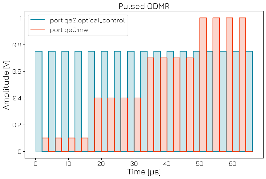
pulsed_odmr_gettable.compiled_schedule.plot_pulse_diagram()

(<Figure size 1000x621 with 1 Axes>,
 <Axes: title={'center': 'Pulsed ODMR'}, xlabel='Time [μs]', ylabel='Amplitude [V]'>)