qblox_scheduler.schedule#

High-level schedule API.

Classes#

Schedule

High-level hybrid schedule.

Module Contents#

class Schedule(name: str, repetitions: int = 1)[source]#

High-level hybrid schedule.

_experiments[source]#

_resources = [][source]#

_schedule_count = None[source]#

_repetitions = 1[source]#

_uses_timeable_repetitions = False[source]#

_duration = None[source]#

clone() → Schedule[source]#: Clone this schedule into a separate independent schedule.

substitute(substitutions: dict[qblox_scheduler.operations.expressions.Expression, qblox_scheduler.operations.expressions.Expression | int | float | complex]) → Schedule[source]#: Substitute matching expressions of operations in this schedule.

property repetitions: int[source]#: Returns the amount of times this schedule should be repeated.

property _experiment: qblox_scheduler.experiments.experiment.Experiment[source]#: Returns the current experiment.

property name: str[source]#: Returns the name of the schedule.

property _timeable_schedules: list[qblox_scheduler.schedules.schedule.TimeableSchedule][source]#: Returns a list of timeable schedules in this schedule.

property _last_timeable_schedule: qblox_scheduler.schedules.schedule.TimeableSchedule | None[source]#: Returns the last timeable schedule in this schedule.

property _timeable_schedule: qblox_scheduler.schedules.schedule.TimeableScheduleBase | None[source]#: Returns the single timeable schedule in this schedule, or None.

get_schedule_duration() → float[source]#

Return total duration of all timeable schedules.

Returns:: schedule_duration : float Duration of current schedule

property duration: float | None[source]#

Determine the cached duration of the schedule.

Will return None if get_schedule_duration() has not been called before.

property data: dict[source]#: The dictionary data of a single contained timeable schedule.

property operations: dict[str, qblox_scheduler.operations.operation.Operation | qblox_scheduler.schedules.schedule.TimeableSchedule][source]#

A dictionary of all unique operations used in the schedule.

This specifies information on what operation to apply where.

The keys correspond to the hash and values are instances of qblox_scheduler.operations.operation.Operation.

property schedulables: dict[str, qblox_scheduler.schedules.schedule.Schedulable][source]#

Ordered dictionary of schedulables describing timing and order of operations.

A schedulable uses timing constraints to constrain the operation in time by specifying the time ("rel_time") between a reference operation and the added operation. The time can be specified with respect to a reference point ("ref_pt"') on the reference operation (:code:”ref_op”) and a reference point on the next added operation (:code:”ref_pt_new”’). A reference point can be either the “start”, “center”, or “end” of an operation. The reference operation ("ref_op") is specified using its label property.

Each item in the list represents a timing constraint and is a dictionary with the following keys:

['label', 'rel_time', 'ref_op', 'ref_pt_new', 'ref_pt', 'operation_id']

The label is used as a unique identifier that can be used as a reference for other operations, the operation_id refers to the hash of an operation in operations.

Note

timing constraints are not intended to be modified directly. Instead use the add()

plot_circuit_diagram(figsize: tuple[int, int] | None = None, ax: matplotlib.axes.Axes | None = None, plot_backend: Literal['mpl'] = 'mpl', timeable_schedule_index: int | None = None) → tuple[matplotlib.figure.Figure | None, matplotlib.axes.Axes | list[matplotlib.axes.Axes]][source]#

Create a circuit diagram visualization of the schedule using the specified plotting backend.

The circuit diagram visualization depicts the schedule at the quantum circuit layer. Because qblox-scheduler uses a hybrid gate-pulse paradigm, operations for which no information is specified at the gate level are visualized using an icon (e.g., a stylized wavy pulse) depending on the information specified at the quantum device layer.

Alias of qblox_scheduler.schedules._visualization.circuit_diagram.circuit_diagram_matplotlib().

Parameters:

figsize – matplotlib figsize.
ax – Axis handle to use for plotting.
plot_backend – Plotting backend to use, currently only ‘mpl’ is supported
timeable_schedule_index – Index of timeable schedule in schedule to plot. If None (the default), will only plot if the schedule contains a single timeable schedule.

Returns:

fig: matplotlib figure object.
ax: matplotlib axis object.

Each gate, pulse, measurement, and any other operation are plotted in the order of execution, but no timing information is provided.

Example

from qblox_scheduler import Schedule
from qblox_scheduler.operations.gate_library import Reset, X90, CZ, Rxy, Measure

sched = Schedule(f"Bell experiment on q0-q1")

sched.add(Reset("q0", "q1"))
sched.add(X90("q0"))
sched.add(X90("q1"), ref_pt="start", rel_time=0)
sched.add(CZ(qC="q0", qT="q1"))
sched.add(Rxy(theta=45, phi=0, qubit="q0") )
sched.add(Measure("q0", acq_index=0))
sched.add(Measure("q1", acq_index=0), ref_pt="start")

sched.plot_circuit_diagram()

(<Figure size 1000x200 with 1 Axes>,
 <Axes: title={'center': 'Bell experiment on q0-q1 schedule 1'}>)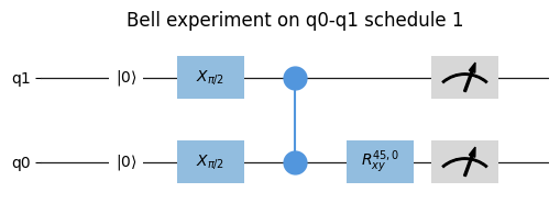

Note

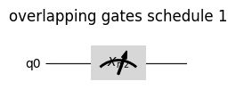
Gates that are started simultaneously on the same qubit will overlap.

from qblox_scheduler import Schedule
from qblox_scheduler.operations.gate_library import X90, Measure

sched = Schedule(f"overlapping gates")

sched.add(X90("q0"))
sched.add(Measure("q0"), ref_pt="start", rel_time=0)
sched.plot_circuit_diagram();

Note

If the pulse’s port address was not found then the pulse will be plotted on the ‘other’ timeline.

plot_pulse_diagram(port_list: list[str] | None = None, sampling_rate: float = 1000000000.0, modulation: Literal['off', 'if', 'clock'] = 'off', modulation_if: float = 0.0, plot_backend: Literal['mpl', 'plotly'] = 'mpl', x_range: tuple[float, float] = (-np.inf, np.inf), combine_waveforms_on_same_port: bool = True, timeable_schedule_index: int | None = None, **backend_kwargs) → tuple[matplotlib.figure.Figure, matplotlib.axes.Axes] | plotly.graph_objects.Figure[source]#

Create a visualization of all the pulses in a schedule using the specified plotting backend.

The pulse diagram visualizes the schedule at the quantum device layer. For this visualization to work, all operations need to have the information present (e.g., pulse info) to represent these on the quantum-circuit level and requires the absolute timing to have been determined. This information is typically added when the quantum-device level compilation is performed.

Alias of qblox_scheduler.schedules._visualization.pulse_diagram.pulse_diagram_matplotlib() and qblox_scheduler.schedules._visualization.pulse_diagram.pulse_diagram_plotly().

Parameters:

port_list – A list of ports to show. If None (default) the first 8 ports encountered in the sequence are used.
modulation – Determines if modulation is included in the visualization.
modulation_if – Modulation frequency used when modulation is set to “if”.
sampling_rate – The time resolution used to sample the schedule in Hz.
plot_backend – Plotting library to use, can either be ‘mpl’ or ‘plotly’.
x_range – The range of the x-axis that is plotted, given as a tuple (left limit, right limit). This can be used to reduce memory usage when plotting a small section of a long pulse sequence. By default (-np.inf, np.inf).
combine_waveforms_on_same_port – By default True. If True, combines all waveforms on the same port into one single waveform. The resulting waveform is the sum of all waveforms on that port (small inaccuracies may occur due to floating point approximation). If False, the waveforms are shown individually.
timeable_schedule_index – Index of timeable schedule in schedule to plot. If None (the default), will only plot if the schedule contains a single timeable schedule.
backend_kwargs – Keyword arguments to be passed on to the plotting backend. The arguments that can be used for either backend can be found in the documentation of qblox_scheduler.schedules._visualization.pulse_diagram.pulse_diagram_matplotlib() and qblox_scheduler.schedules._visualization.pulse_diagram.pulse_diagram_plotly().

Returns:

Union[tuple[Figure, Axes], plotly.graph_objects.Figure] the plot

Example

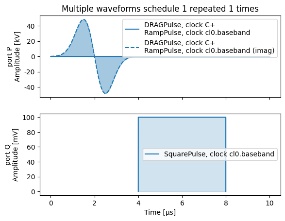
A simple plot with matplotlib can be created as follows:

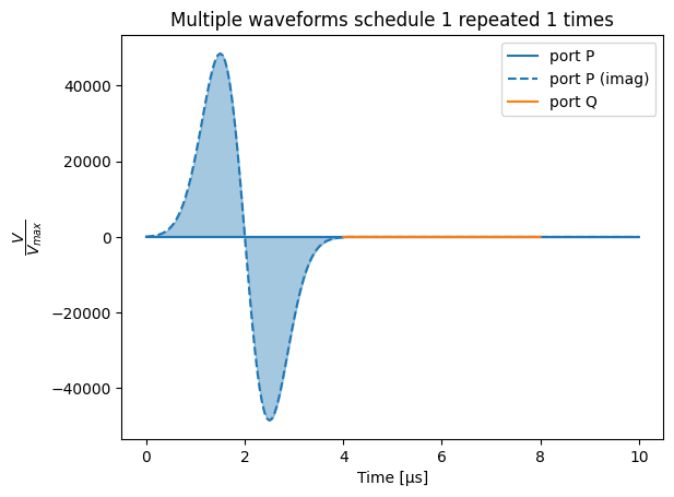
from qblox_scheduler.backends.graph_compilation import SerialCompiler
from qblox_scheduler.device_under_test.quantum_device import QuantumDevice
from qblox_scheduler.operations.pulse_library import (
    DRAGPulse, SquarePulse, RampPulse, VoltageOffset,
)
from qblox_scheduler.resources import ClockResource

schedule = Schedule("Multiple waveforms")
schedule.add(DRAGPulse(amplitude=0.2, beta=0.2, phase=0, duration=4e-6, port="P", clock="C"))
schedule.add(RampPulse(amp=0.2, offset=0.0, duration=6e-6, port="P"))
schedule.add(SquarePulse(amp=0.1, duration=4e-6, port="Q"), ref_pt='start')
schedule.add_resource(ClockResource(name="C", freq=4e9))

quantum_device = QuantumDevice("quantum_device")
device_compiler = SerialCompiler("Device compiler", quantum_device)
compiled_schedule = device_compiler.compile(schedule)

_ = compiled_schedule.plot_pulse_diagram(sampling_rate=20e6)

The backend can be changed to the plotly backend by specifying the plot_backend=plotly argument. With the plotly backend, pulse diagrams include a separate plot for each port/clock combination:

_ = compiled_schedule.plot_pulse_diagram(sampling_rate=20e6, plot_backend='plotly')

The same can be achieved in the default plot_backend (matplotlib) by passing the keyword argument multiple_subplots=True:

_ = compiled_schedule.plot_pulse_diagram(sampling_rate=20e6, multiple_subplots=True)

By default, waveforms overlapping in time on the same port are shown separately:

schedule = Schedule("Overlapping waveforms")
schedule.add(VoltageOffset(offset_path_I=0.25, offset_path_Q=0.0, port="Q"))
schedule.add(SquarePulse(amp=0.1, duration=4e-6, port="Q"), rel_time=2e-6)
schedule.add(VoltageOffset(offset_path_I=0.0, offset_path_Q=0.0, port="Q"), ref_pt="start", rel_time=2e-6)

compiled_schedule = device_compiler.compile(schedule)

_ = compiled_schedule.plot_pulse_diagram(sampling_rate=20e6)

This behaviour can be changed with the parameter combine_waveforms_on_same_port:

_ = compiled_schedule.plot_pulse_diagram(sampling_rate=20e6, combine_waveforms_on_same_port=True)

property timing_table: pandas.io.formats.style.Styler[source]#

A styled pandas dataframe containing the absolute timing of pulses and acquisitions in a schedule.

This table is constructed based on the abs_time key in the schedulables. This requires the timing to have been determined.

The table consists of the following columns:

operation: a repr of Operation corresponding to the pulse/acquisition.
waveform_op_id: an id corresponding to each pulse/acquisition inside an Operation.
port: the port the pulse/acquisition is to be played/acquired on.
clock: the clock used to (de)modulate the pulse/acquisition.
abs_time: the absolute time the pulse/acquisition is scheduled to start.
duration: the duration of the pulse/acquisition that is scheduled.
is_acquisition: whether the pulse/acquisition is an acquisition or not (type numpy.bool_).
wf_idx: the waveform index of the pulse/acquisition belonging to the Operation.
operation_hash: the unique hash corresponding to the Schedulable that the pulse/acquisition belongs to.

Example

schedule = Schedule("demo timing table")
schedule.add(Reset("q0", "q4"))
schedule.add(X("q0"))
schedule.add(Y("q4"))
schedule.add(Measure("q0", acq_channel=0))
schedule.add(Measure("q4", acq_channel=1))

compiled_schedule = compiler.compile(schedule)
compiled_schedule.timing_table

	waveform_op_id	port	clock	abs_time	duration	is_acquisition	operation	wf_idx	operation_hash
0	Reset('q0','q4')_acq_0	None	cl0.baseband	0.0 ns	200,000.0 ns	False	Reset('q0','q4')	0	4661729798253199648
1	Reset('q0','q4')_acq_1	None	cl0.baseband	0.0 ns	200,000.0 ns	False	Reset('q0','q4')	1	4661729798253199648
2	X(qubit='q0')_acq_0	q0:mw	q0.01	200,000.0 ns	20.0 ns	False	X(qubit='q0')	0	1485574851275385533
3	Y(qubit='q4')_acq_0	q4:mw	q4.01	200,020.0 ns	20.0 ns	False	Y(qubit='q4')	0	-703654793022745977
4	ResetClockPhase(clock='q0.ro',t0=0)_acq_0	None	q0.ro	200,040.0 ns	0.0 ns	False	ResetClockPhase(clock='q0.ro',t0=0)	0	6835988571585172774
5	VoltageOffset(offset_path_I=0.25,offset_path_Q=0,port='q0:res',clock='q0.ro',t0=0,reference_magnitude=None)_acq_0	q0:res	q0.ro	200,040.0 ns	0.0 ns	False	VoltageOffset(offset_path_I=0.25,offset_path_Q=0,port='q0:res',clock='q0.ro',t0=0,reference_magnitude=None)	0	8020950697660214393
8	SSBIntegrationComplex(port='q0:res',clock='q0.ro',duration=1e-06,acq_channel=0,coords=None,acq_index=None,bin_mode='average_append',phase=0,t0=1e-07)_acq_0	q0:res	q0.ro	200,140.0 ns	1,000.0 ns	True	SSBIntegrationComplex(port='q0:res',clock='q0.ro',duration=1e-06,acq_channel=0,coords=None,acq_index=None,bin_mode='average_append',phase=0,t0=1e-07)	0	7287739078375794900
6	VoltageOffset(offset_path_I=0.0,offset_path_Q=0.0,port='q0:res',clock='q0.ro',t0=0,reference_magnitude=None)_acq_0	q0:res	q0.ro	200,336.0 ns	0.0 ns	False	VoltageOffset(offset_path_I=0.0,offset_path_Q=0.0,port='q0:res',clock='q0.ro',t0=0,reference_magnitude=None)	0	4936325873099508079
7	SquarePulse(amp=0.25,duration=4e-09,port='q0:res',clock='q0.ro',reference_magnitude=None,t0=0)_acq_0	q0:res	q0.ro	200,336.0 ns	4.0 ns	False	SquarePulse(amp=0.25,duration=4e-09,port='q0:res',clock='q0.ro',reference_magnitude=None,t0=0)	0	-3933578044769354881
9	ResetClockPhase(clock='q4.ro',t0=0)_acq_0	None	q4.ro	201,140.0 ns	0.0 ns	False	ResetClockPhase(clock='q4.ro',t0=0)	0	-5750836303515347058
10	VoltageOffset(offset_path_I=0.25,offset_path_Q=0,port='q4:res',clock='q4.ro',t0=0,reference_magnitude=None)_acq_0	q4:res	q4.ro	201,140.0 ns	0.0 ns	False	VoltageOffset(offset_path_I=0.25,offset_path_Q=0,port='q4:res',clock='q4.ro',t0=0,reference_magnitude=None)	0	6078352190798997592
13	SSBIntegrationComplex(port='q4:res',clock='q4.ro',duration=1e-06,acq_channel=1,coords=None,acq_index=None,bin_mode='average_append',phase=0,t0=1e-07)_acq_0	q4:res	q4.ro	201,240.0 ns	1,000.0 ns	True	SSBIntegrationComplex(port='q4:res',clock='q4.ro',duration=1e-06,acq_channel=1,coords=None,acq_index=None,bin_mode='average_append',phase=0,t0=1e-07)	0	6860129394656206594
11	VoltageOffset(offset_path_I=0.0,offset_path_Q=0.0,port='q4:res',clock='q4.ro',t0=0,reference_magnitude=None)_acq_0	q4:res	q4.ro	201,436.0 ns	0.0 ns	False	VoltageOffset(offset_path_I=0.0,offset_path_Q=0.0,port='q4:res',clock='q4.ro',t0=0,reference_magnitude=None)	0	-4484542811907451762
12	SquarePulse(amp=0.25,duration=4e-09,port='q4:res',clock='q4.ro',reference_magnitude=None,t0=0)_acq_0	q4:res	q4.ro	201,436.0 ns	4.0 ns	False	SquarePulse(amp=0.25,duration=4e-09,port='q4:res',clock='q4.ro',reference_magnitude=None,t0=0)	0	5203982912090299319

Returns:

: styled_timing_table, a pandas Styler containing a dataframe with an overview of the timing of the pulses and acquisitions present in the schedule. The dataframe can be accessed through the .data attribute of the Styler.

Raises:

ValueError – When the absolute timing has not been determined during compilation.

_add_timeable_schedule(timeable_schedule: qblox_scheduler.schedules.schedule.TimeableSchedule) → None[source]#

_get_current_timeable_schedule() → qblox_scheduler.schedules.schedule.TimeableSchedule | None[source]#

_get_timeable_schedule() → qblox_scheduler.schedules.schedule.TimeableSchedule[source]#

get_used_port_clocks() → set[tuple[str, str]][source]#

Extracts which port-clock combinations are used in this schedule.

Returns:

: All (port, clock) combinations that operations in this schedule uses

add_resources(resources_list: list) → None[source]#: Add wrapper for adding multiple resources.

add_resource(resource: qblox_scheduler.resources.Resource) → None[source]#: Add a resource such as a channel or device element to the schedule.

declare(dtype: qblox_scheduler.operations.expressions.DType) → qblox_scheduler.operations.variables.Variable[source]#

Declare a new variable.

Parameters:: dtype – The data type of the variable.

add(operation: Schedule | qblox_scheduler.operations.operation.Operation | qblox_scheduler.schedules.schedule.TimeableSchedule | qblox_scheduler.experiments.experiment.Step, rel_time: float | qblox_scheduler.operations.expressions.Expression = 0, ref_op: qblox_scheduler.schedules.schedule.Schedulable | str | None = None, ref_pt: qblox_scheduler.schedules.schedule.OperationReferencePoint | None = None, ref_pt_new: qblox_scheduler.schedules.schedule.OperationReferencePoint | None = None, label: str | None = None) → qblox_scheduler.schedules.schedule.Schedulable | None[source]#: Add step, operation or timeable schedule to this schedule.

_add_schedule(schedule: Schedule, rel_time: float | qblox_scheduler.operations.expressions.Expression = 0, ref_op: qblox_scheduler.schedules.schedule.Schedulable | str | None = None, ref_pt: qblox_scheduler.schedules.schedule.OperationReferencePoint | None = None, ref_pt_new: qblox_scheduler.schedules.schedule.OperationReferencePoint | None = None, label: str | None = None) → qblox_scheduler.schedules.schedule.Schedulable | None[source]#

loop(domain: qblox_scheduler.operations.loop_domains.LinearDomain, rel_time: float = 0, ref_op: qblox_scheduler.schedules.schedule.Schedulable | str | None = None, ref_pt: qblox_scheduler.schedules.schedule.OperationReferencePoint | None = None, ref_pt_new: qblox_scheduler.schedules.schedule.OperationReferencePoint | None = None, strategy: qblox_scheduler.operations.control_flow_library.LoopStrategy | None = None) → collections.abc.Iterator[qblox_scheduler.operations.variables.Variable][source]#

loop(*domains: qblox_scheduler.operations.loop_domains.LinearDomain, rel_time: float = 0, ref_op: qblox_scheduler.schedules.schedule.Schedulable | str | None = None, ref_pt: qblox_scheduler.schedules.schedule.OperationReferencePoint | None = None, ref_pt_new: qblox_scheduler.schedules.schedule.OperationReferencePoint | None = None, strategy: qblox_scheduler.operations.control_flow_library.LoopStrategy | None = None) → collections.abc.Iterator[list[qblox_scheduler.operations.variables.Variable]]

Add a loop operation to the schedule, using a with-statement.

Every operation added while the context manager is active, will be added to the loop body.

Example:

sched = Schedule()
with sched.loop(linspace(start_amp, start_amp + 1.0, 11, dtype=DType.AMP)) as amp:
    sched.add(SquarePulse(amp=amp, duration=100e-9, port="q0:mw", clock="q0.01"))

Parameters:

domain – The object that describes the domain to be looped over.
domains – Optional extra domains that will be looped over in parallel, in a zip-like fashion.
rel_time – relative time between the reference operation and the added operation. the time is the time between the “ref_pt” in the reference operation and “ref_pt_new” of the operation that is added.
ref_op – reference schedulable. If set to None, will default to the last added operation.
ref_pt – reference point in reference operation must be one of "start", "center", "end", or None; in case of None, _determine_absolute_timing() assumes "end".
ref_pt_new – reference point in added operation must be one of "start", "center", "end", or None; in case of None, _determine_absolute_timing() assumes "start".
strategy – Strategy to use for implementing this loop, will default to None indicating no preference.

Yields:

variables – The Variable objects that are created for each domain.