Interleaved RB/ProbeT1#

This notebook implements a combined randomized benchmarking (RB) and \(T_1\) coherence measurement designed to probe the correlation between gate fidelity and energy relaxation within a single, hardware-efficient schedule.

\(T_1\) is reported to fluctuate on timescales ranging from milliseconds to hours [1], and these fluctuations can have a significant impact on gate fidelities in superconducting qubits. However, standard RB experiments typically take too long to capture these fluctuations in real time, making it difficult to directly correlate changes in \(T_1\) with changes in gate performance. The interleaved RB/T1 schedule addresses this by embedding a rapid \(T_1\) estimation within the RB sequence itself.

For each seed, a Clifford sequence of fixed length is applied to the qubit, followed by a measurement. Using a single sequence length (rather than sweeping the number of Cliffords \(m\)) makes the experiment fast enough to track fluctuations over time. The measured overlap with the target state is then used to extract an estimate of the depolarizing parameter \(p\) by inverting the RB decay model. Immediately after the RB measurements for all seeds, a \(T_1\) estimation is performed by implementing the probe_t1 schedule. The qubit is prepared in |1⟩ , allowed to relax for a fixed wait time \(\tau \approx T_1\), which is where the exponential decay is the most sensitive to fluctuations.

[1]:

import matplotlib.pyplot as plt
import numpy as np
from dependencies.analysis_utils import ProbeT1Analysis, RBAnalysis, T1Analysis
from dependencies.randomized_benchmarking.utils import (
    InterleavedRBT1Analysis,
    interleaved_randomized_benchmarking_and_t1,
    randomized_benchmarking_schedule,
)
from matplotlib import image as mpimg
from xarray import open_dataset

from qblox_scheduler import HardwareAgent, Schedule
from qblox_scheduler.operations import Measure, Reset, X
from qblox_scheduler.operations.acquisition_library import BinMode
from qblox_scheduler.operations.expressions import DType
from qblox_scheduler.operations.loop_domains import arange

Generating hash table for SingleQubitClifford.
Hash table generated.
Generating hash table for TwoQubitCliffordCZ.
Hash table generated.
Generating hash table for TwoQubitCliffordZX.
Hash table generated.

/.venv/lib/python3.14/site-packages/quantify_core/visualization/instrument_monitor.py:13: QCoDeSDeprecationWarning: The `qcodes.utils.helpers` module is deprecated. Please consult the api documentation at https://microsoft.github.io/Qcodes/api/index.html for alternatives.
  from qcodes.utils.helpers import strip_attrs

Testing decompositions.
Test passed.

Setup#

The hardware agent manages the connection to the instrument and ensures that pulses and acquisitions happen over the appropriate input and output channels of the Cluster. The cell below creates an instance of the HardwareAgent based on the hardware- and device-under-test configuration files in the ./dependencies/configs folder, allowing us to start doing measurements. We also define some convenient aliases to use throughout our measurements. For a more thorough discussion of the hardware- and device-under-test configuration files, check out this tutorial.

[2]:

# Set up hardware agent, this automatically connects to the instrument
hw_agent = HardwareAgent(
    hardware_configuration="./dependencies/configs/hw_config.json",
    quantum_device_configuration="./dependencies/configs/dut_config.json",
)

# convenience aliases
q0 = hw_agent.quantum_device.get_element("q0")  # Qubits 0 and 2 are measured using QRM-RF + QCM-RF
q2 = hw_agent.quantum_device.get_element("q2")
q3 = hw_agent.quantum_device.get_element("q3")  # Qubit 3 is measured using QRC

cluster = hw_agent.get_clusters()["cluster"]
hw_options = hw_agent.hardware_configuration.hardware_options
qubit = q0

/.venv/lib/python3.14/site-packages/qblox_scheduler/qblox/hardware_agent.py:499: UserWarning: cluster: Trying to instantiate cluster with ip 'None'.Creating a dummy cluster.
  warnings.warn(

Calibration: SPAM errors#

The fast \(T_1\) and fast interleaved \(T_1\) and RB measurements repeatedly measure a binary outcome \(|0⟩\) or \(|1⟩\) after a fixed duration or fixed number of gates. To extract \(T_1\) and fidelity values from these, we need to first calibrate the SPAM errors. SPAM can be measured using a single-shot readout experiment. Here we assume that these have been measured before.

[3]:

p01 = 0.1  # False negative SPAM error: the probability of measuring 0 when preparing 1
p10 = 0.05  # False positive SPAM error: the probability of measuring 1 when preparing 0

Calibration: traditional \(T_1\) and RB measurements#

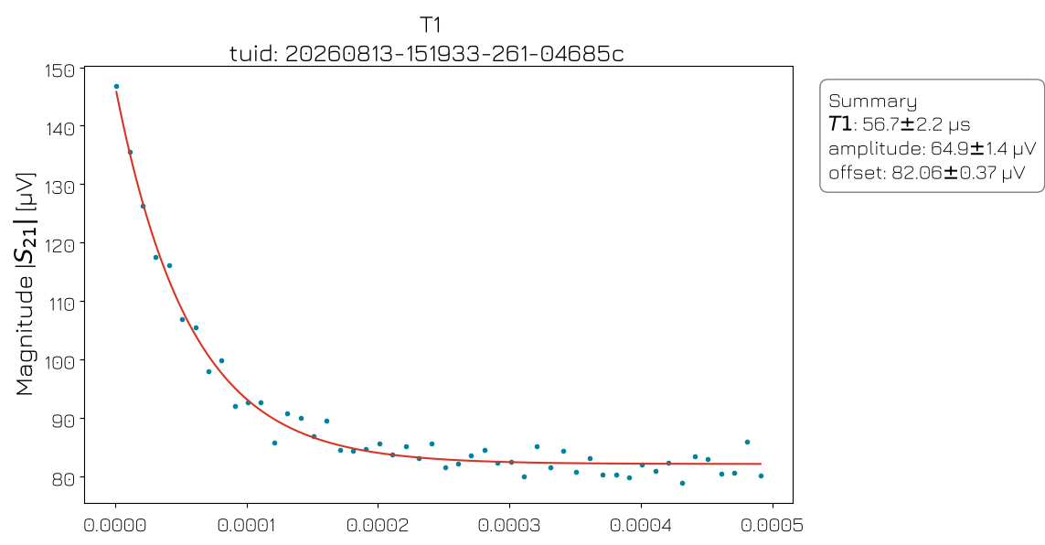
First, a normal \(T_1\) decay measurement is performed to get the most recent value of \(T_1\). This is then used as the waiting time τ in the ProbeT1 schedule.

[4]:

# Start with a $T_1$ analysis to set the tau needed for the ProbeT1 experiment

tau_start = 1e-6  # s
tau_stop = 500e-6  # s
tau_step = 10e-6  # s

repetitions = 1000

t1_sched = Schedule(name="t1_experiment")

with (
    t1_sched.loop(arange(0, repetitions, 1, DType.NUMBER)),
    t1_sched.loop(arange(start=tau_start, stop=tau_stop, step=tau_step, dtype=DType.TIME)) as tau,
):
    t1_sched.add(Reset(qubit.name))
    # Prepare |1>
    t1_sched.add(X(qubit=qubit.name))
    # Measure after time tau
    t1_sched.add(Measure(qubit.name, coords={"tau": tau}, acq_channel="S_21"), rel_time=tau)

# Execute the experiment
t1_data = hw_agent.run(t1_sched)
if cluster.is_dummy:
    example_data = open_dataset("./dependencies/datasets/probe_t1_n.hdf5", engine="h5netcdf")
    t1_data = t1_data.update({"S_21": example_data.S_21})


t1_analysis = T1Analysis(t1_data).run()
t1_analysis.display_figs_mpl()

t1 = t1_analysis.quantities_of_interest["T1"].nominal_value

../../../_images/applications_superconducting_fixed_frequency_transmon_301_interleaved_rb_t1_8_0.png

Then, a standard RB schedule is performed to extract the most recent fit of the decay curve, from which the optimal Clifford gate sequence length \(m^*\) can be derived.

[5]:

# Run test RB with a fixed gate sequence length
lengths = np.arange(0, 40, 5)
seeds = np.random.randint(0, 2**31 - 1, size=10, dtype=np.int32)

repetitions = 10

sched = randomized_benchmarking_schedule(
    qubit.name,
    lengths=lengths,
    repetitions=repetitions,
    seeds=seeds,
)

# Execute the experiment
rb_data = hw_agent.run(sched)
if cluster.is_dummy:
    example_data = open_dataset(
        "./dependencies/datasets/single_qubit_randomized_benchmarking.hdf5", engine="h5netcdf"
    )
    rb_data.update({"S_21": example_data.S_21, "calibration": example_data.calibration})

rb_analysis = RBAnalysis(rb_data).run()
rb_analysis.display_figs_mpl()
rb_analysis.quantities_of_interest

/.venv/lib/python3.14/site-packages/numpy/lib/_function_base_impl.py:682: ComplexWarning: Casting complex values to real discards the imaginary part
  a = asarray(a, dtype=dtype, order=order)
/.venv/lib/python3.14/site-packages/matplotlib/cbook.py:1719: ComplexWarning: Casting complex values to real discards the imaginary part
  return math.isfinite(val)
/.venv/lib/python3.14/site-packages/matplotlib/collections.py:200: ComplexWarning: Casting complex values to real discards the imaginary part
  offsets = np.asanyarray(offsets, float)

[5]:

{'alpha': np.float64(0.9675848343006597),
 'error_per_clifford': np.float64(0.016207582849670166),
 'error_per_clifford_error': np.float64(0.004284565638857489),
 'prefactor': np.float64(0.362756581541486),
 'prefactor_error': np.float64(0.022126169752721053)}

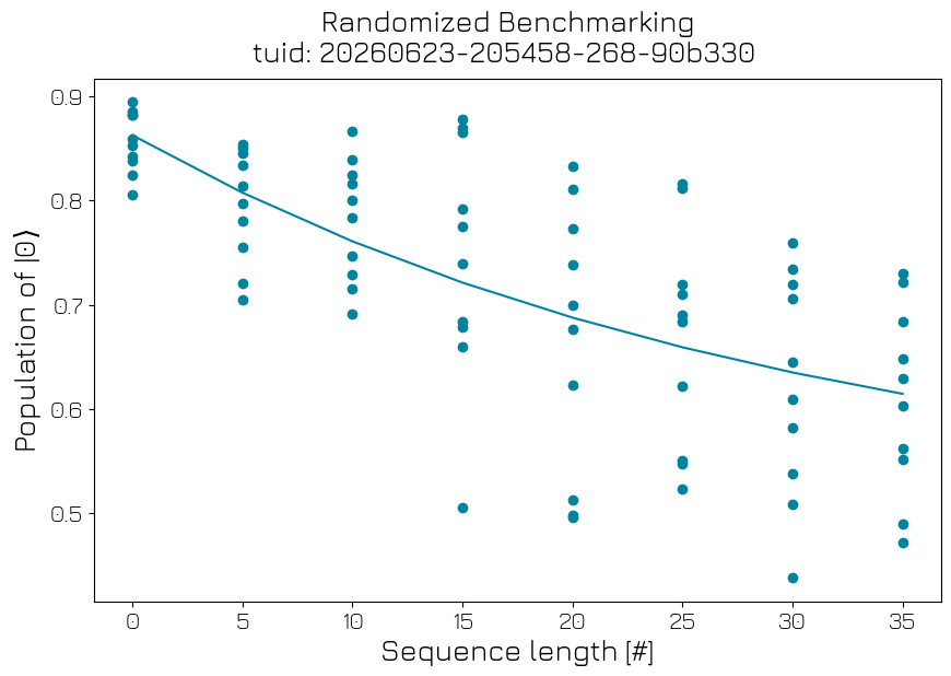
../../../_images/applications_superconducting_fixed_frequency_transmon_301_interleaved_rb_t1_10_2.png

The optimal sequence length can be calculated using the formula \(m^* = -1 / \log(p)\), where \(p\) is the depolarizing parameter extracted from the RB fit. This sequence length corresponds to the point where the RB decay curve is most sensitive to fluctuations in gate fidelity.

[6]:

# Find the optimal sequence length m* for the RB experiment
p = rb_analysis.quantities_of_interest["alpha"]

m_star = int(-1 / np.log(p))
print("Optimal sequence length m* =", m_star)

Optimal sequence length m* = 30

`ProbeT1` schedule and analysis#

First, the ProbeT1 schedule is constructed and executed to get a high-temporal-resolution estimate of \(T_1\) fluctuations.

[7]:

# # `ProbeT1` schedule

probe_t1 = Schedule(name="t1_experiment")
repetitions = 1e4

# This schedule needs to run for around a few minutes at least, so that fluctuations on lower frequencies can also be observed
with (
    probe_t1.loop(arange(0, repetitions, 1, DType.NUMBER)),
):
    probe_t1.add(Reset(qubit.name))
    # Prepare |1>
    probe_t1.add(X(qubit=qubit.name))
    # Measure after time tau
    probe_t1.add(
        Measure(
            qubit.name,
            acq_protocol="ThresholdedAcquisition",
            acq_channel="bits_t1",
            bin_mode=BinMode.APPEND,
        ),
        ref_pt="start",
        rel_time=round(t1, 9),
    )

# Execute the experiment
t1_data = hw_agent.run(probe_t1)
if cluster.is_dummy:
    example_data = open_dataset("./dependencies/datasets/probe_t1_c.hdf5", engine="h5netcdf")
    t1_data = t1_data.update({"bits_t1": example_data.y0})

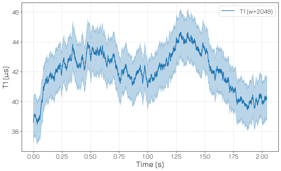
The ProbeT1 schedule can measure \(T_1\) with higher temporal resolution than a regular \(T_1\) schedule. Since \(T_1\) fluctuates more rapidly than a standard RB schedule, it is important to assess how much of these fluctuations occur at frequencies higher than those sampled by the RB schedule to make meaningful statements about their correlation. Therefore, a power spectral density (PSD) analysis is performed to visualize the distribution of fluctuations across frequency bands. Combined with the RB schedule frequency, this provides an estimate of how much of the \(T_1\) variability is captured by the interleaved experiment.

[8]:

# Sampling frequency (approx). If reset_time is known:
reset_time = 200e-6
cycle_time = reset_time + t1  # seconds
psd_fs = 1.0 / cycle_time

# Instantiate and run analysis
analysis = ProbeT1Analysis(
    dataset=t1_data,
    tau=t1,
    psd_fs=psd_fs,
    segment_length=2**11,
    trace_window=2**11,  # use high-res window for time trace
    nperseg=2**11,
    p01=p01,
    p10=p10,
    bridge_bend=2.0,
    time_rb=1e-3,
).run()

analysis.display_figs_mpl()

/builds/0/tmpvceunga6/dependencies/analysis_utils.py:464: UserWarning: nperseg=2048 is greater than signal length max(len(x), len(y)) = 4, using nperseg = 4
  f_low, p_low = welch(
/builds/0/tmpvceunga6/dependencies/analysis_utils.py:594: UserWarning: Glyph 8209 (\N{NON-BREAKING HYPHEN}) missing from font(s) Jura.
  fig.tight_layout()
/.venv/lib/python3.14/site-packages/qblox_scheduler/analysis/base_analysis.py:665: UserWarning: Glyph 8209 (\N{NON-BREAKING HYPHEN}) missing from font(s) Jura.
  fig.savefig(f"{filename}.{form}", bbox_inches="tight", dpi=dpi)

../../../_images/applications_superconducting_fixed_frequency_transmon_301_interleaved_rb_t1_16_1.png

/.venv/lib/python3.14/site-packages/IPython/core/pylabtools.py:170: UserWarning: Glyph 8209 (\N{NON-BREAKING HYPHEN}) missing from font(s) Jura.
  fig.canvas.print_figure(bytes_io, **kw)

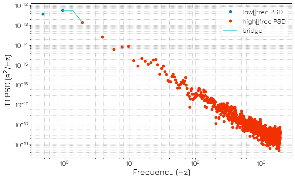
../../../_images/applications_superconducting_fixed_frequency_transmon_301_interleaved_rb_t1_16_3.png

The PSD plot shows how the \(T_1\) fluctuations are distributed across frequencies, while the time trace provides a direct visualization of the \(T_1\) dynamics over the course of the experiment.

Interleaved RB/ProbeT1 schedule and analysis#

With the optimal sequence length \(m^*\) and the \(T_1\) value, the interleaved RB/T1 schedule can be constructed. The RB part consists of a loop over seeds where for each seed, a Clifford sequence of length \(m^*\) (optimal sequence length) is applied followed by a measurement. After all seeds have been measured, a probe \(T_1\) estimation is performed by preparing the qubit in |1⟩, waiting for a time \(\tau \approx T_1\) (this is the most sensitive time point in the exponential decay), and then measuring via thresholded acquisition to get a binary outcome indicating whether the qubit decayed to |0⟩ or not.

[9]:

seeds = np.random.randint(0, 2**31 - 1, size=10, dtype=np.int32)
schedule = interleaved_randomized_benchmarking_and_t1(
    qubit.name,
    length=m_star,
    seeds=seeds,
    repetitions=50,
    t1=t1,
    n_t1_points=1,
)

i_data = hw_agent.run(schedule)

if cluster.is_dummy:
    example_data = open_dataset("./dependencies/datasets/probe_rb.hdf5", engine="h5netcdf")
    i_data = i_data.update(
        {
            "y0": example_data.y0,
        }
    )

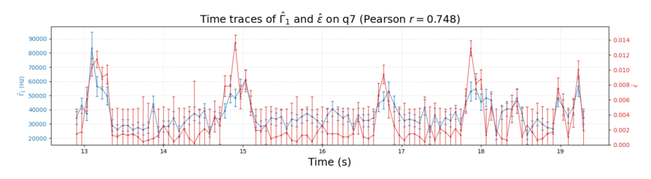
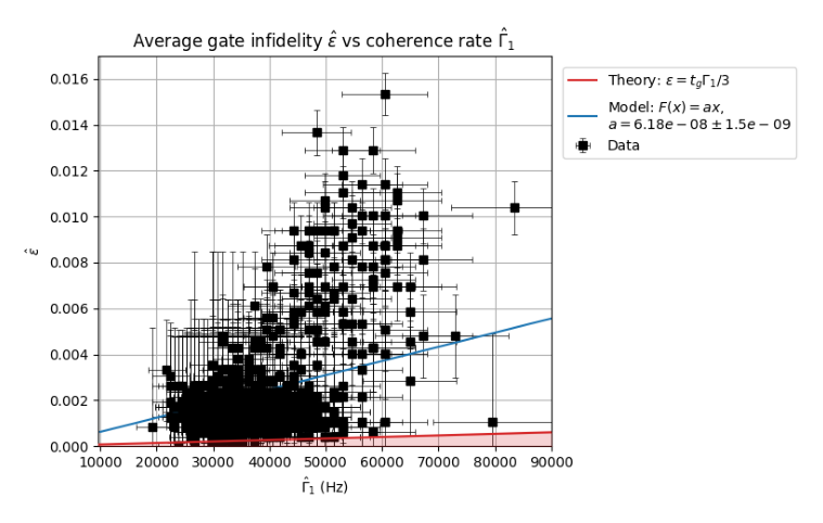
Now to analyze the interleaved RB/ProbeT1. The analysis provides a timetrace of both the gate fidelity and the \(T_1\) for each repetition of the schedule. From these points, the (Pearson) correlation coefficient can be calculated, which provides insight into how much the gate fidelity is correlated with fluctuations in \(T_1\). Additionally, the PSD provides us with an estimate of the variance of \(T_1\) itself over the relevant time scale, which contributes to the error bar of our \(T_1\) (or \(\Gamma_1=1/T_1\)) estimate.

[10]:

analysis = InterleavedRBT1Analysis(
    dataset=i_data,
    a=rb_analysis.quantities_of_interest["prefactor"],
    m_length=m_star,
    seeds=seeds,
    tau=t1,
    n_t1_points=1,
    repetitions=50,
    p01=p01,
    p10=p10,
    t1_var=analysis.quantities_of_interest["T1_avg_variance"],
).run()

if cluster.is_dummy:
    image1 = mpimg.imread("./figures/interleavedrb_t1_trace.png")
    image2 = mpimg.imread("./figures/interleavedrb_t1_scatter.png")
    plt.figure(figsize=(12, 6))
    plt.imshow(image1)
    plt.axis("off")
    plt.show()
    plt.figure(figsize=(12, 6))
    plt.imshow(image2)
    plt.axis("off")
    plt.show()
else:
    analysis.display_figs_mpl()

../../../_images/applications_superconducting_fixed_frequency_transmon_301_interleaved_rb_t1_21_0.png

../../../_images/applications_superconducting_fixed_frequency_transmon_301_interleaved_rb_t1_21_1.png

The example data was collected by using the Quantum Inspire platform [2] to run experiments on the Tuna-9 processor, a chip with 9 flux-tunable transmon qubits developed and maintained by the DiCarlo lab at TU Delft.

Conclusion#

The interleaved RB/\(T_1\) experiment probes how fast fluctuations in the energy relaxation time \(T_1\) co-vary with the average single-qubit gate fidelity, as quantified by the Pearson correlation coefficient \(r\). A large positive \(r\) indicates that, within the frequency band accessible to the RB/\(T_1\) schedule, longer \(T_1\) is systematically associated with higher gate fidelity, whereas a small \(r\) implies that variations in \(T_1\) explain only a minor part of the observed gate-error fluctuations.

References#

[1] Berritta, Fabrizio, et al. “Real-time adaptive tracking of fluctuating relaxation rates in superconducting qubits.” Physical Review X 16.1 (2026): 011025

[2] Thorsten Last et al. “Quantum Inspire: QuTech’s platform for co-development and collaboration in quantum computing”. In: Novel patterning technologies for semiconductors, MEMS/NEMS and MOEMS 2020. Vol. 11324. SPIE. 2020, pp. 49–59.