
See also
A Jupyter notebook version of this tutorial can be downloaded here.

Golden-section search#
The golden-section search (GSS) is an iterative numerical method used to find the extremum (minimum or maximum) of a unimodal function within a specified interval. Unlike gradient-based methods it does not require derivative information, making it highly robust against the noise that is typically present in (superconducting) quantum systems.
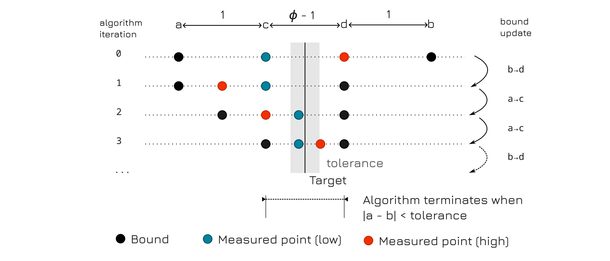
The algorithm systematically narrows the range of the search by probing the interior of the interval at two specific points. By maintaining a constant ratio between the lengths of the sub-intervals, the method ensures that each step reduces the search space efficiently.
The technique derives its name and efficiency from the golden ratio, denoted by \(\phi\) and defined as:
See the figure below for an example of how the algorithm converges to a minimum value.
Spectroscopic peak / dip finding#
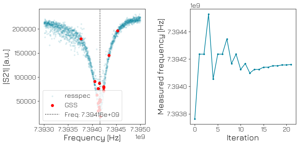
In this application example, we employ the Golden-Section Search (GSS) algorithm to pinpoint the resonance frequency of a readout resonator coupled to a superconducting transmon qubit. This feature shows up as a dip in the magnitude of the transmission spectrum.
Using GSS we can find this minimum without performing a dense and time-consuming frequency sweep. Furthermore, this implementation does not require any post-measurement analysis as the final readout frequency is immediately stored inside a register within the sequencer. This drastically reduces the duration of the qubit calibration cycle.
[1]:
import matplotlib.pyplot as plt
import numpy as np
import xarray as xr
from qcodes.instrument import find_or_create_instrument

from qblox_instruments import Cluster, ClusterType

# Ensure that frequency values are 16-bit signed integers by setting maximum allowed parameter values.
F_RESOLUTION = 1e3  # 1 kHz maximum allowed frequency resolution
MAX_F_RANGE = 8000 * F_RESOLUTION
Connect to cluster#
[2]:
cluster_ip = None
cluster: Cluster = find_or_create_instrument(
    Cluster,
    recreate=True,
    name="cluster0",
    identifier=cluster_ip,
    dummy_cfg=(
        {
            13: ClusterType.CLUSTER_QRM_RF,
        }
        if cluster_ip is None
        else None
    ),
)
cluster.reset()

# Notation shorthands
mod = cluster.module13
seq = mod.sequencer0
Set up LINQ#
For information on how to set up the LINQ routing, see this tutorial. For general information about LINQ, check out the user guide.
[3]:
LINQ_ID = 50
cluster.set_cmm_route(id_=[LINQ_ID], targets=[seq])
Set up qcodes parameters#
Configure the cluster’s qcodes for the experiment. These in general depend on the setup and should be calibrated before running the algorithm.
[4]:
lo_frequency = 7.8e9  # LO frequency output tone. Should be <400MHz from target frequency.
ro_att = 20  # QRM_RF output attenuation in dB
in_att = 0  # QRM_RF input attenuation in dB
[5]:
mod.disconnect_outputs()
mod.disconnect_inputs()

# Configure readout sequencer
seq.connect_sequencer("io0")
seq.mod_en_awg(True)
seq.demod_en_acq(True)
seq.marker_ovr_en(True)
seq.marker_ovr_value(3)

mod.out0_att(ro_att)
mod.in0_att(in_att)
mod.out0_in0_lo_freq(lo_frequency)
Define golden-section search algorithm#
Python#
The q1asm implementation of the golden-section algorithm can be daunting. To understand how it works, it can help to look at the python code below (from wikipedia).
def gss(f, a, b, tolerance=1e-5) -> float:
    """
    Define Golden-section search to find the minimum of f on [a,b].

    * f: a strictly unimodal function on [a,b]

    Example:
    >>> def f(x): return (x - 2) ** 2
    >>> x = gss(f, 1, 5)
    >>> print(f"{x:.5f}")
    2.00000

    """
    invphi = (np.sqrt(5) - 1) / 2  # 1 / phi
    while b - a > tolerance:
        c = b - (b - a) * invphi
        d = a + (b - a) * invphi
        if f(c) < f(d):
            b = d
        else:  # f(c) > f(d) to find the maximum
            a = c

    return (b + a) / 2
q1asm#
The code below implements the golden-section search algorithm for finding the dip in a resonator connected to a superconducting transmon qubit. To make it suitable for other applications, the user is only required to modify the measure_point subroutine. The “main” routine implementing the logic of shrinking the window can stay as is.
[6]:
def golden_section(
    tolerance: float,
    f_center: float,
    f_range: float,
    ro_duration: int,
    linq_channel: int,
    max_shots: int,
) -> str:
    """Create a golden-section search algorithm in q1asm."""
    if f_range > MAX_F_RANGE:
        raise ValueError(
            f"Frequency range {f_range} larger than maximum allowed value {MAX_F_RANGE}!"
        )

    invphi = int((1 << 15) * (np.sqrt(5) - 1) / 2)  # Pre-compute golden ratio

    qrm_program = f"""
        # --- Initialization ---
        move            {int(4 * f_center)}, R1                 # Frequency center
        move            {int(4 * tolerance / F_RESOLUTION)}, R0 # Convergence condition
        move            {-int(2 * f_range / F_RESOLUTION)}, R4  # lower bound (a) -> R4
        move            {int(2 * f_range / F_RESOLUTION)}, R5   # upper bound (b) -> R5
        move            0, R24                                  # Acquisition index
        fb_acq_iq_id    {linq_channel}, 12                      # Enable IQ feedback
        fb_acq_iq_shift 8, 8
        set_awg_gain    32000, 0

        check_conv:
                sub             R5, R4, R6                  # (b) - (a) -> R6
                nop
                cmp             R6, R0                      # Compare against tolerance
                jl              @stop_sequencer             # Exit if converged

                # --- Calculate Probe Points ---
                muls16          R6, {invphi}, R7            # ((b) - (a)) * invphi -> R7
                nop
                asr             R7, 15, R7                  # Normalize shift
                nop
                sub             R5, R7, R8                  # left probe (c) -> R8
                add             R4, R7, R9                  # right probe (d) -> R9
                nop

                # --- Measure Point (c) ---
                move            R8, R15                     # Pass R8 to measurement routine
                move            @measure_point_ret_c, R27   # Pass R27 to measurement routine
                jmp             @measure_point
        measure_point_ret_c:
                move            R13, R16                    # Store result (c) in R16

                # --- Measure Point (d) ---
                move            R9, R15                     # Pass R9 to measurement routine
                move            @measure_point_ret_d, R27   # Pass R27 to measurement routine
                jmp             @measure_point
        measure_point_ret_d:
                move            R13, R17                    # Store result (d) in R17

                # --- Update Bounds ---
                cmp             R24, {max_shots}            # Safety break
                jge             @stop_sequencer

                cmp             R16, R17                    # Compare magnitude at (c) and (d)
                jl              @pick_left                  # If s21(c) < s21(d) -> left interval

        pick_right:                                         # Else -> right interval
                move            R8, R4                      # (c) -> (a)
                jmp             @check_conv

        pick_left:
                move            R9, R5                      # (d) -> (b)
                jmp             @check_conv

        stop_sequencer:
                add             R4, R5, R28                 # Minimum at: ((b) + (a)) / 2 + freq_cen
                nop
                muls16          R28, {int(F_RESOLUTION)}, R28
                nop
                asr             R28, 1, R28
                nop
                add             R28, R1, R28                # Frequency of minimum stored in R28

                stop            4

        # =========================================================
        # SUBROUTINE: measure_point
        # Input: R15 (relative freq offset)
        # Input: R27 (return line number)
        # Output: R13 (Magnitude squared: I^2 + Q^2)
        # =========================================================
        measure_point:
                # --- Set the frequency for the next measurement ---
                muls16          R15, {int(F_RESOLUTION)}, R15
                nop
                add             R15, R1, R15                # Apply center offset
                nop
                set_freq        R15

                set_awg_offs    2500, 0                     # Pulse ON
                upd_param       4
                acquire         0, R24, 4

                # --- A long wait loop to measure the transmission of the resonator ---
                move            {int(ro_duration // 65535)}, R31
        wait_loop:
                wait            65535
                sub             R31, 1, R31
                jnz             @wait_loop
                wait            {int(ro_duration % 65535)}

                set_awg_offs    0, 0                        # Pulse OFF
                upd_param       4
                add             1, R24, R24                 # Increment shot index

                wait            2000                        # Latency buffer
                fb_pop_data     {linq_channel}, R23         # I
                fb_pop_data     {linq_channel}, R10         # Q

                muls32          R23, R23, R11, R20          # I^2
                nop
                muls32          R10, R10, R12, R21          # Q^2
                nop
                add             R20, R21, R13               # Final R13 = Power
                nop

                jmp             R27                         # Return to main routine
        """
    return qrm_program
Resonator spectroscopy#
Below is a q1asm program that executes a “normal” resonator spectroscopy experiment following the same code implementation described above. This will allow us to make a comparison between the two algorithms and verify that the GSS algorithm is working as expected.
[7]:
def resspec(
    f_center: float,  # target - LO [Hz]
    f_range: float,  # [Hz]
    ro_duration: int,  # [ns]
) -> str:
    """Create resonator spectroscopy program."""
    n_shots = f_range // F_RESOLUTION
    program = f"""
        move                        {int(4 * f_center)}, R1                     # Frequency center
        move                        {-int(2 * f_range / F_RESOLUTION)}, R4      # lower bound -> R4
        move                        {int(2 * f_range / F_RESOLUTION)}, R5       # upper bound -> R5
        move            0, R24

        move            R4, R8
        set_awg_gain    32000,0

        muls16          R8, {int(F_RESOLUTION)}, R8                 # Calculate NCO frequency
        nop
        add             R8, R1, R8                                  # Add center frequency
        nop

        increment:
            set_freq                R8                                      # Set the measurement frequency

        measure_point:
            set_awg_offs    2500, 0                                 # Pulse ON
            upd_param       4
            acquire         0, R24, 4

            # --- Long Wait Loop ---
            move            {int((ro_duration - 4) // 65535)}, R31
        wait_loop:
            wait            65535
            sub             R31, 1, R31
            jnz             @wait_loop
            wait            {int((ro_duration - 4) % 65535)}

            set_awg_offs    0, 0                                    # Pulse OFF
            upd_param       4
            add             1, R24, R24                             # Increment shot index
            add             R8, {int(4 * F_RESOLUTION)}, R8

            cmp             R24, {int(n_shots)}
            jl              @increment

        stop_sequencer:
            stop
    """
    return program
Analysis#
Below are classes to analyze the results of the resonator spectroscopy and golden-section search. Frequencies at which the GSS algorithm was executed are determined by retracing the algorithm’s steps based on the measured data.
[8]:
def calc_s21(dataset: xr.Dataset) -> xr.Dataset:
    """Calculate transmitted signal S21 from raw dataset."""
    dataset["s21"] = np.abs(dataset.path0 + 1j * dataset.path1)
    return dataset.dropna(dim="sample")
[9]:
def set_resspec_axis(dataset: xr.Dataset, f_center: float, f_range: float) -> xr.Dataset:
    """Change the axis of the resspec to frequency."""
    a = f_center - (f_range // 2)
    b = f_center + (f_range // 2)
    f_points = np.linspace(a, b, dataset.s21.size)

    temp = dataset.assign_coords(freq=(["sample"], f_points))
    return temp.swap_dims({"sample": "freq"})
[10]:
def calc_freqs(dataset: xr.Dataset, f_center: float, f_range: float) -> xr.Dataset:
    """Recalculate the frequencies at which the GSS algorithm measured."""
    invphi = (np.sqrt(5) - 1) / 2  # 1 / phi

    a = f_center - (f_range // 2)
    b = f_center + (f_range // 2)
    f_points = []

    for i in range(dataset.s21.size // 2):
        f_points.append(b - (b - a) * invphi)
        f_points.append(a + (b - a) * invphi)

        if dataset.s21[i * 2] ** 2 < dataset.s21[i * 2 + 1] ** 2:
            b = a + (b - a) * invphi
        else:
            a = b - (b - a) * invphi

    temp = dataset.assign_coords(freq=(["sample"], f_points))
    return temp.swap_dims({"sample": "freq"})
Upload sequence#
[11]:
# Generic settings
f_range = 2_000_000  # Hz
f_center = 7_394_000_000  # Hz
ro_duration = 1_000_000  # ns
seq.integration_length_acq(ro_duration)

# GSS settings
tolerance = 5_000  # Hz
max_shots = 1000
[12]:
# Run a resonator spectroscopy experiment
seq.sequence(
    {
        "waveforms": {},
        "acquisitions": {"ground": {"index": 0, "num_bins": int(f_range // F_RESOLUTION)}},
        "weights": {},
        "program": resspec(
            f_center=int(f_center - lo_frequency),  # Hz
            f_range=f_range,  # Hz
            ro_duration=ro_duration,
        ),
    }
)
seq.arm_sequencer()
seq.start_sequencer()
seq.get_sequencer_status(timeout=1)

# Create an xarray dataset for data manipulation.
raw_data = seq.get_acquisitions()["ground"]["acquisition"]["bins"]
resspec_ds = xr.Dataset(
    data_vars={
        "path0": (["sample"], raw_data["integration"]["path0"]),
        "path1": (["sample"], raw_data["integration"]["path1"]),
    },
    coords={"sample": np.arange(len(raw_data["threshold"]))},
)
[13]:
# Run a golden section experiment
seq.sequence(
    {
        "waveforms": {},
        "acquisitions": {"ground": {"index": 0, "num_bins": max_shots}},
        "weights": {},
        "program": golden_section(
            tolerance=tolerance,  # Hz
            f_center=int(f_center - lo_frequency),  # Hz
            f_range=f_range,  # Hz
            ro_duration=ro_duration,
            max_shots=max_shots,
            linq_channel=LINQ_ID,
        ),
    }
)
seq.arm_sequencer()
seq.start_sequencer()
seq.get_sequencer_status(timeout=1)

# Create an xarray dataset for data manipulation.
raw_data = seq.get_acquisitions()["ground"]["acquisition"]["bins"]
gss_ds = xr.Dataset(
    data_vars={
        "path0": (["sample"], raw_data["integration"]["path0"]),
        "path1": (["sample"], raw_data["integration"]["path1"]),
    },
    coords={"sample": np.arange(len(raw_data["threshold"]))},
)
[14]:
if cluster.is_dummy:
    gss_ds_processed = xr.load_dataset("dependencies/datasets/golden_section.h5", engine="netcdf4")
    resspec_ds_processed = xr.load_dataset(
        "dependencies/datasets/golden_section_resspec.h5", engine="netcdf4"
    )
else:
    gss_ds_processed = gss_ds.pipe(calc_s21).pipe(calc_freqs, f_center, f_range)
    resspec_ds_processed = resspec_ds.pipe(calc_s21).pipe(set_resspec_axis, f_center, f_range)
Plotting#
[15]:
# Calculate the frequency as the average frequency of the last two measurement points
gss_freq = (gss_ds_processed.freq[-1] + gss_ds_processed.freq[-2]) / 2

fig, ax = plt.subplots(ncols=2, nrows=1, figsize=(10, 5))

ax[0].scatter(
    resspec_ds_processed.freq,
    np.abs(resspec_ds_processed.s21),
    marker=".",
    alpha=0.1,
    label="resspec",
)
ax[0].scatter(
    gss_ds_processed.freq, np.abs(gss_ds_processed.s21), marker="o", ls="-", c="r", label="GSS"
)
ax[0].axvline(gss_freq, color="k", ls=":", label=f"Freq: {gss_freq:.5e}")
ax[0].set_xlabel("Frequency [Hz]")
ax[0].set_ylabel("|S21| [a.u.]")
ax[0].legend()

ax[1].plot(range(gss_ds_processed.freq.size), gss_ds_processed.freq, marker=".")
ax[1].set_xlabel("Iteration")
ax[1].set_ylabel("Measured frequency [Hz]")

plt.tight_layout()
plt.show()