See also

A Jupyter notebook version of this tutorial can be downloaded here.

Flux-tunable transmons tuneup

This notebook contains all the required steps for the tuneup of flux-tunable transmons. We show how to connect to the instrument as well as example schedules for tuneup and benchmarking of this chip architecture.

import matplotlib.pyplot as plt
import numpy as np
from dependencies.analysis_utils import (
    EchoAnalysis,
    PunchoutAnalysis,
    QubitSpectroscopyAnalysis,
    RabiAnalysis,
    RamseyAnalysis,
    RBAnalysis,
    ResonatorFluxSpectroscopyAnalysis,
    ResonatorSpectroscopyAnalysis,
    SSROAnalysis,
    T1Analysis,
    TimeOfFlightAnalysis,
)
from dependencies.randomized_benchmarking.clifford_group import TwoQubitCliffordCZ
from dependencies.randomized_benchmarking.utils import randomized_benchmarking_schedule
from xarray import open_dataset

from qblox_scheduler import HardwareAgent, Schedule
from qblox_scheduler.analysis.helpers import acq_coords_to_dims
from qblox_scheduler.experiments import SetHardwareOption, SetParameter
from qblox_scheduler.operations import (
    X90,
    IdlePulse,
    Measure,
    Reset,
    SetClockFrequency,
    SquarePulse,
    VoltageOffset,
    X,
)
from qblox_scheduler.operations.expressions import DType
from qblox_scheduler.operations.loop_domains import arange, linspace

Generating hash table for SingleQubitClifford.
Hash table generated.
Generating hash table for TwoQubitCliffordCZ.
Hash table generated.
Generating hash table for TwoQubitCliffordZX.
Hash table generated.
Testing decompositions.
Test passed.

Setup

The hardware agent manages the connection to the instrument and ensures that pulses and acquisitions happen over the appropriate input and output channels of the Cluster. The cell below creates an instance of the HardwareAgent based on the hardware- and device-under-test configuration files in the ./dependencies/configs folder, allowing us to start doing measurements. We also define some convenient aliases to use throughout our measurements. For a more thorough discussion of the hardware- and device-under-test configuration files, check out this tutorial.

# Set up hardware agent, this automatically connects to the instrument
hw_agent = HardwareAgent(
    hardware_configuration="./dependencies/configs/hw_config.json",
    quantum_device_configuration="./dependencies/configs/dut_config.json",
)

# convenience aliases
q0 = hw_agent.quantum_device.get_element("q0")
q2 = hw_agent.quantum_device.get_element("q2")
cluster = hw_agent.get_clusters()["cluster"]
hw_options = hw_agent.hardware_configuration.hardware_options
qubit = q0

/builds/0/.venv/lib/python3.10/site-packages/qblox_scheduler/qblox/hardware_agent.py:460: UserWarning: cluster: Trying to instantiate cluster with ip 'None'.Creating a dummy cluster.
  warnings.warn(

Time of flight

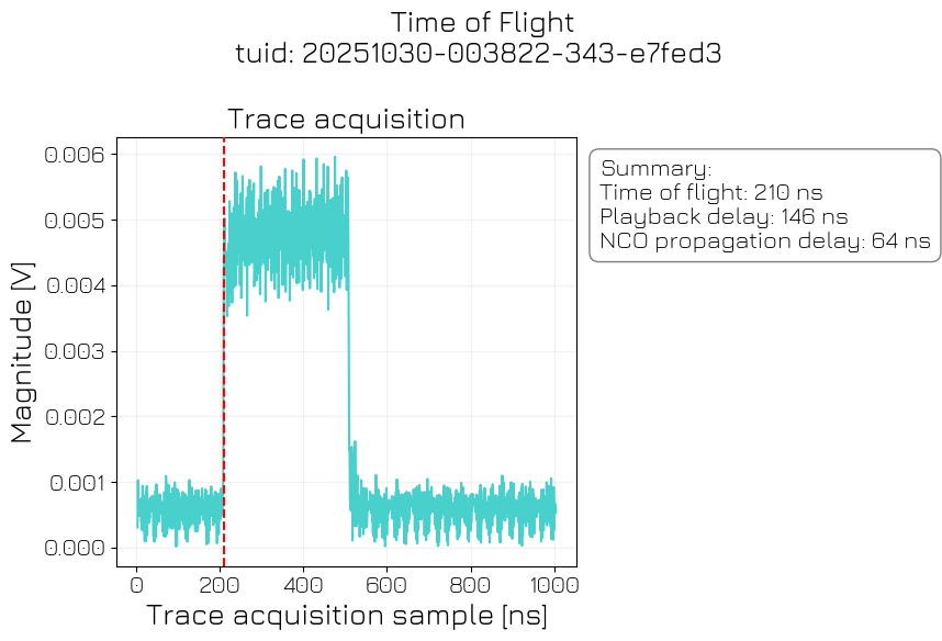
Prior to the start of quantum experiments, it is crucial to calibrate the delay between sending a measurement pulse and beginning the acquisition on the instrument. This delay should be equal to the time it takes for the readout signal to travel through the fridge and is determined by the length of the cables. For the experiment a square pulse is played over the output of the readout line, while a trace acquisition is done. The time at which the pulse is detected on the acquisition path is determined to be the acquisition delay. This also allows us to set the NCO propagation delay, which corrects for the phase accumulated during the time of flight.

Experiment settings

# Pulse settings
pulse_attenuation = 0  # dB
pulse_amplitude = 1  # a.u.
pulse_frequency_detuning = 100e6  # Hz
pulse_duration = 300e-9  # ns
acquisition_duration = 1e-6  # Hz

repetitions = 1000

Experiment schedule

# Set pulse attenuation
prior_att = hw_options.output_att[f"{qubit.name}:res-{qubit.name}.ro"]
hw_options.output_att[f"{qubit.name}:res-{qubit.name}.ro"] = pulse_attenuation

tof_sched = Schedule("time_of_flight")
tof_sched.add(
    SetClockFrequency(
        clock=qubit.name + ".ro",
        clock_freq_new=qubit.clock_freqs.readout - pulse_frequency_detuning,
    )  # Detune clock 100MHz from expected resonance frequency
)
tof_sched.add(IdlePulse(4e-9))
with tof_sched.loop(arange(0, repetitions, 1, DType.NUMBER)):
    tof_sched.add(
        Measure(
            qubit.name,
            acq_protocol="Trace",
            pulse_duration=pulse_duration,
            acq_duration=acquisition_duration,
            acq_channel="S_21",
            acq_delay=0,
        )
    )

# Execute the experiment
tof_data = hw_agent.run(tof_sched)
if cluster.is_dummy:
    example_data = open_dataset("./dependencies/datasets/time_of_flight.hdf5", engine="h5netcdf")
    tof_data = tof_data.update({"S_21": example_data.S_21})

# Reset attenuation
hw_options.output_att[f"{qubit.name}:res-{qubit.name}.ro"] = prior_att

Analyze the experiment

tof_analysis = TimeOfFlightAnalysis(tof_data).run()
tof_analysis.display_figs_mpl()

Post-run

qubit.measure.acq_delay = tof_analysis.quantities_of_interest["tof"]

# Set the NCO propagation delay of the readout line.
cluster.module4.sequencer0.nco_prop_delay_comp_en(True)
cluster.module4.sequencer0.nco_prop_delay_comp(
    tof_analysis.quantities_of_interest["nco_prop_delay"]
)

Resonator Spectroscopy

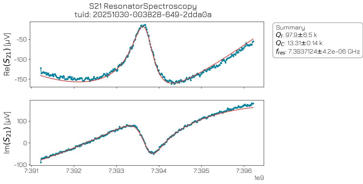
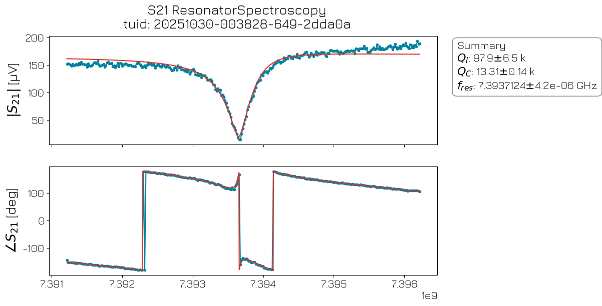
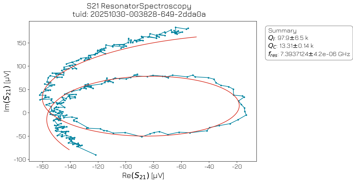
In a resonator spectroscopy experiment, we sweep the frequency of a microwave tone applied to the readout line. When the drive tone frequency matches the resonator’s resonance frequency, a change in the amplitude and/or phase of the reflected signal is observed.

Experiment settings

# Frequency settings
frequency_center = qubit.clock_freqs.readout  # Hz
frequency_width = 5e6  # Hz
frequency_npoints = 300

repetitions = 1000

Experiment schedule

spec_sched = Schedule("resonator_spectroscopy")
with (
    spec_sched.loop(arange(0, repetitions, 1, DType.NUMBER)),
    spec_sched.loop(
        linspace(
            start=frequency_center - frequency_width / 2,
            stop=frequency_center + frequency_width / 2,
            num=frequency_npoints,
            dtype=DType.FREQUENCY,
        )
    ) as freq,
):
    spec_sched.add(Measure(qubit.name, freq=freq, coords={"frequency": freq}, acq_channel="S_21"))
    spec_sched.add(IdlePulse(10e-6))  # Let the resonator decay

# Execute the experiment
rs_data = hw_agent.run(spec_sched)
if cluster.is_dummy:
    example_data = open_dataset(
        "./dependencies/datasets/resonator_spectroscopy.hdf5", engine="h5netcdf"
    )
    tof_data = rs_data.update({"S_21": example_data.S_21})

Analyze the experiment

resspec_analysis = ResonatorSpectroscopyAnalysis(rs_data).run()
resspec_analysis.display_figs_mpl()

Post-run

# Update device config
qubit.clock_freqs.readout = resspec_analysis.quantities_of_interest["fr"].nominal_value

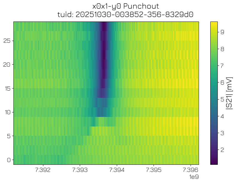
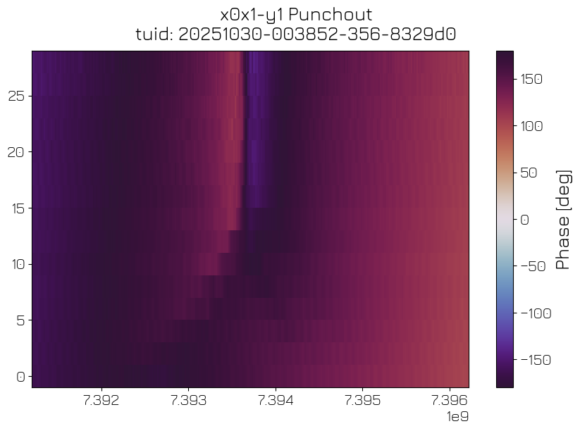
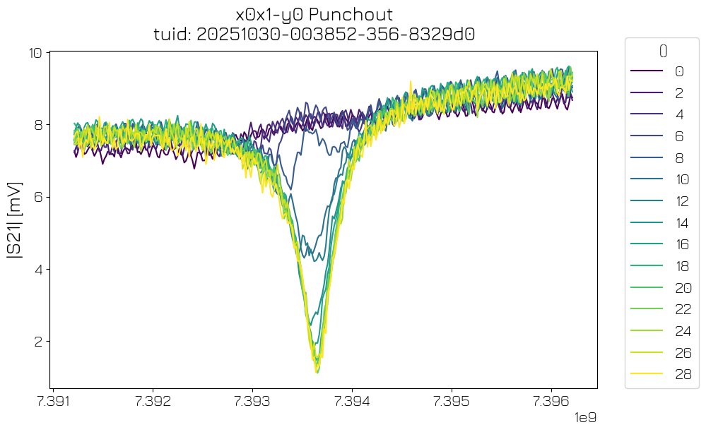
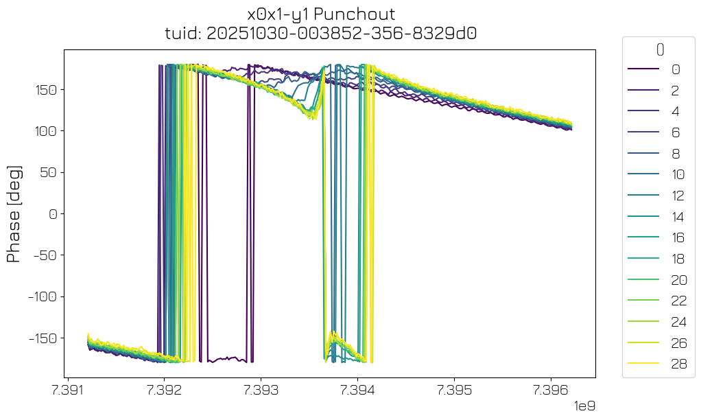
Resonator punchout

To verify the presence of a qubit coupled to the resonator, and to optimize the readout signal-to-noise ratio (SNR) while preventing back-action on the qubit, we perform a “punchout” experiment by sweeping the attenuation of the microwave tone over resonator spectroscopy traces. In the high-power regime the resonator responds at its bare frequency, while at the low-power regime the resonator frequency is dressed by the coupling to the qubit. The crossover between the two is called “resonator punchout” (Blais et al., 2021: https://arxiv.org/abs/2005.12667).

Experiment settings

# Frequency settings
frequency_center = qubit.clock_freqs.readout  # Hz
frequency_width = 5e6  # Hz
frequency_npoints = 300

# Attenuation settings
att_start = 0  # dB
att_stop = 30  # dB
att_step = 2  # dB

repetitions = 100

Experiment schedule

po_sched = Schedule("resonator_punchout")

with po_sched.loop(
    arange(start=att_start, stop=att_stop, step=att_step, dtype=DType.NUMBER)
) as amp:
    # Set output attenuation
    po_sched.add(SetHardwareOption("output_att", amp, f"{qubit.name}:res-{qubit.name}.ro"))
    with (
        po_sched.loop(arange(0, repetitions, 1, DType.NUMBER)),
        po_sched.loop(
            linspace(
                start=frequency_center - frequency_width / 2,
                stop=frequency_center + frequency_width / 2,
                num=frequency_npoints,
                dtype=DType.FREQUENCY,
            )
        ) as freq,
    ):
        po_sched.add(
            Measure(
                qubit.name,
                freq=freq,
                coords={"frequency": freq, "amp": amp},
                acq_channel="S_21",
            )
        )
        po_sched.add(IdlePulse(10e-6))  # Let the resonator decay

# Execute the experiment
po_data = hw_agent.run(po_sched)
if cluster.is_dummy:
    example_data = open_dataset(
        "./dependencies/datasets/resonator_punchout.hdf5", engine="h5netcdf"
    )
    po_data = po_data.update({"S_21": example_data.S_21})

/builds/0/.venv/lib/python3.10/site-packages/pydantic/main.py:464: UserWarning: Pydantic serializer warnings:
  PydanticSerializationUnexpectedValue(Expected `int` - serialized value may not be as expected [field_name='output_att', input_value=0.0, input_type=float])
  return self.__pydantic_serializer__.to_python(
/builds/0/.venv/lib/python3.10/site-packages/pydantic/main.py:464: UserWarning: Pydantic serializer warnings:
  PydanticSerializationUnexpectedValue(Expected `int` - serialized value may not be as expected [field_name='output_att', input_value=2.0, input_type=float])
  return self.__pydantic_serializer__.to_python(
/builds/0/.venv/lib/python3.10/site-packages/pydantic/main.py:464: UserWarning: Pydantic serializer warnings:
  PydanticSerializationUnexpectedValue(Expected `int` - serialized value may not be as expected [field_name='output_att', input_value=4.0, input_type=float])
  return self.__pydantic_serializer__.to_python(
/builds/0/.venv/lib/python3.10/site-packages/pydantic/main.py:464: UserWarning: Pydantic serializer warnings:
  PydanticSerializationUnexpectedValue(Expected `int` - serialized value may not be as expected [field_name='output_att', input_value=6.0, input_type=float])
  return self.__pydantic_serializer__.to_python(
/builds/0/.venv/lib/python3.10/site-packages/pydantic/main.py:464: UserWarning: Pydantic serializer warnings:
  PydanticSerializationUnexpectedValue(Expected `int` - serialized value may not be as expected [field_name='output_att', input_value=8.0, input_type=float])
  return self.__pydantic_serializer__.to_python(
/builds/0/.venv/lib/python3.10/site-packages/pydantic/main.py:464: UserWarning: Pydantic serializer warnings:
  PydanticSerializationUnexpectedValue(Expected `int` - serialized value may not be as expected [field_name='output_att', input_value=10.0, input_type=float])
  return self.__pydantic_serializer__.to_python(
/builds/0/.venv/lib/python3.10/site-packages/pydantic/main.py:464: UserWarning: Pydantic serializer warnings:
  PydanticSerializationUnexpectedValue(Expected `int` - serialized value may not be as expected [field_name='output_att', input_value=12.0, input_type=float])
  return self.__pydantic_serializer__.to_python(
/builds/0/.venv/lib/python3.10/site-packages/pydantic/main.py:464: UserWarning: Pydantic serializer warnings:
  PydanticSerializationUnexpectedValue(Expected `int` - serialized value may not be as expected [field_name='output_att', input_value=14.0, input_type=float])
  return self.__pydantic_serializer__.to_python(
/builds/0/.venv/lib/python3.10/site-packages/pydantic/main.py:464: UserWarning: Pydantic serializer warnings:
  PydanticSerializationUnexpectedValue(Expected `int` - serialized value may not be as expected [field_name='output_att', input_value=16.0, input_type=float])
  return self.__pydantic_serializer__.to_python(
/builds/0/.venv/lib/python3.10/site-packages/pydantic/main.py:464: UserWarning: Pydantic serializer warnings:
  PydanticSerializationUnexpectedValue(Expected `int` - serialized value may not be as expected [field_name='output_att', input_value=18.0, input_type=float])
  return self.__pydantic_serializer__.to_python(
/builds/0/.venv/lib/python3.10/site-packages/pydantic/main.py:464: UserWarning: Pydantic serializer warnings:
  PydanticSerializationUnexpectedValue(Expected `int` - serialized value may not be as expected [field_name='output_att', input_value=20.0, input_type=float])
  return self.__pydantic_serializer__.to_python(
/builds/0/.venv/lib/python3.10/site-packages/pydantic/main.py:464: UserWarning: Pydantic serializer warnings:
  PydanticSerializationUnexpectedValue(Expected `int` - serialized value may not be as expected [field_name='output_att', input_value=22.0, input_type=float])
  return self.__pydantic_serializer__.to_python(
/builds/0/.venv/lib/python3.10/site-packages/pydantic/main.py:464: UserWarning: Pydantic serializer warnings:
  PydanticSerializationUnexpectedValue(Expected `int` - serialized value may not be as expected [field_name='output_att', input_value=24.0, input_type=float])
  return self.__pydantic_serializer__.to_python(
/builds/0/.venv/lib/python3.10/site-packages/pydantic/main.py:464: UserWarning: Pydantic serializer warnings:
  PydanticSerializationUnexpectedValue(Expected `int` - serialized value may not be as expected [field_name='output_att', input_value=26.0, input_type=float])
  return self.__pydantic_serializer__.to_python(
/builds/0/.venv/lib/python3.10/site-packages/pydantic/main.py:464: UserWarning: Pydantic serializer warnings:
  PydanticSerializationUnexpectedValue(Expected `int` - serialized value may not be as expected [field_name='output_att', input_value=28.0, input_type=float])
  return self.__pydantic_serializer__.to_python(

Analyze the experiment

punchout_analysis = PunchoutAnalysis(po_data).run()
punchout_analysis.display_figs_mpl()

Post-run

# Update the device config
hw_options.output_att[f"{qubit.name}:res-{qubit.name}.ro"] = 24

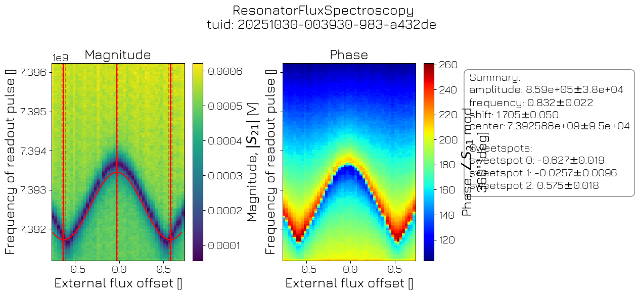
Resonator flux spectroscopy

By changing the magnetic flux through a flux-tunable transmon, the frequency of the qubit’s |0⟩ → |1⟩ transition can be controlled. While idling, the qubit is commonly kept at its “flux-sweetspot”, where it is less susceptible to magnetic field noise. To ensure that the qubit is at the sweetspot, the voltage bias over the flux line should be calibrated. To do this we use dependence of the resonator dispersive (Lamb) shift on the qubit frequency, such that any change in the |0⟩ → |1⟩ transition frequency results in a change of the readout frequency. For the experiment, the voltage bias over the flux line is swept while performing resonator spectroscopy experiments. This allows for a course calibration of the necessary bias voltage.

Experiment settings

# Frequency settings
frequency_center = qubit.clock_freqs.readout  # Hz
frequency_width = 5e6  # Hz
frequency_npoints = 150

# Flux settings
flux_start = -0.75  # V
flux_stop = 0.75  # V
flux_step = 0.030  # V

repetitions = 100

Before sweeping the voltage over the flux port, we define a new parameter that represents the voltage output of the instrument. This allows us to ensure that the flux bias changes gradually, to avoid that the frequency of the qubit changes due to sudden voltage changes over the flux line. This uses Qcodes under the hood.

flux_offset = cluster.module14.out0_offset  # Flux port of q0
flux_offset.inter_delay = 100e-9  # Delay time between consecutive set operations.
flux_offset.step = 0.3e-3  # Stepsize in V that this Parameter uses during set operation.

flux_offset.get()  # Get before setting to avoid jumps.
flux_offset.set(0.0)  # V

Experiment schedule

flux_res_sched = Schedule("flux_resonator_spectroscopy")

with flux_res_sched.loop(
    arange(start=flux_start, stop=flux_stop, step=flux_step, dtype=DType.AMPLITUDE)
) as amp:
    # Set the flux offset voltage.
    flux_res_sched.add(SetParameter(flux_offset, amp))
    with (
        flux_res_sched.loop(arange(0, repetitions, 1, DType.NUMBER)),
        flux_res_sched.loop(
            linspace(
                start=frequency_center - frequency_width / 2,
                stop=frequency_center + frequency_width / 2,
                num=frequency_npoints,
                dtype=DType.FREQUENCY,
            )
        ) as freq,
    ):
        flux_res_sched.add(
            Measure(
                qubit.name,
                freq=freq,
                coords={"frequency": freq, "amplitude": amp},
                acq_channel="S_21",
            )
        )
        flux_res_sched.add(IdlePulse(10e-6))  # Let the resonator decay

# Execute the experiment
flux_res_data = hw_agent.run(flux_res_sched)
if cluster.is_dummy:
    example_data = open_dataset(
        "./dependencies/datasets/flux_resonator_spectroscopy.hdf5", engine="h5netcdf"
    )
    flux_res_data = flux_res_data.update({"S_21": example_data.S_21})

Analyze the experiment

flux_resspec_analysis = ResonatorFluxSpectroscopyAnalysis(flux_res_data).run()
flux_resspec_analysis.display_figs_mpl()

Post-run

# Update flux offset
flux_offset(flux_resspec_analysis.quantities_of_interest["sweetspot_1"].nominal_value)

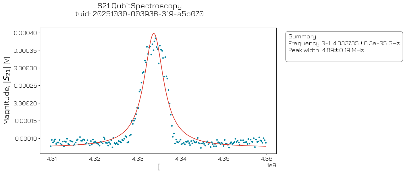
Qubit spectroscopy

Two-tone spectroscopy is used to determine the transition frequency between the |0⟩ and |1⟩ states. In addition to the tone played on the readout line, a second microwave tone is played on the drive line of the qubit. When the qubit drive frequency becomes resonant with the qubit’s |0⟩ → |1⟩ transition, the qubit absorbs energy and changes its state. This change is then detected in the amplitude of the readout signal at the previously calibrated resonator frequency.

Experiment settings

# Drive attenuation settings. Should be an even number <= 30
drive_att = 30  # dB

# Drive frequency settings
f01_center = qubit.clock_freqs.f01  # Hz
f01_width = 50e6  # Hz
f01_npoints = 200

repetitions = 1e3

Experiment schedule

two_tone_sched = Schedule("two_tone_spectroscopy")
# Set the drive attenuation for the experiment
two_tone_sched.add(SetHardwareOption("output_att", drive_att, f"{qubit.name}:mw-{qubit.name}.01"))

with two_tone_sched.loop(
    linspace(
        start=f01_center - f01_width / 2,
        stop=f01_center + f01_width / 2,
        num=f01_npoints,
        dtype=DType.FREQUENCY,
    )
) as freq:
    # Set a constant tone out of the drive line to probe the f01 frequency
    two_tone_sched.add(VoltageOffset(0.01, 0, port=qubit.ports.microwave, clock=qubit.name + ".01"))
    two_tone_sched.add(SetClockFrequency(clock=qubit.name + ".01", clock_freq_new=freq))

    two_tone_sched.add(Reset(qubit.name))
    with two_tone_sched.loop(arange(0, repetitions, 1, DType.NUMBER)):
        two_tone_sched.add(Measure(qubit.name, coords={"frequency": freq}, acq_channel="S_21"))

    # Reset drive line voltage to 0
    two_tone_sched.add(VoltageOffset(0, 0, port=qubit.ports.microwave, clock=qubit.name + ".01"))
    two_tone_sched.add(IdlePulse(4e-9))

# Execute the experiment
qs_data = hw_agent.run(two_tone_sched)
if cluster.is_dummy:
    example_data = open_dataset(
        "./dependencies/datasets/qubit_spectroscopy.hdf5", engine="h5netcdf"
    )
    qs_data = qs_data.update({"S_21": example_data.S_21})

Analyze the experiment

qs_analysis = QubitSpectroscopyAnalysis(qs_data).run()
qs_analysis.display_figs_mpl()

Post-run

# Update device config
qubit.clock_freqs.f01 = qs_analysis.quantities_of_interest["frequency_01"].nominal_value

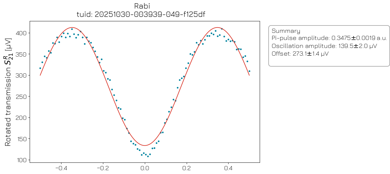
Rabi

After determining the qubit’s |0⟩ → |1⟩ transition frequency, a Rabi experiment is performed to calibrate the required microwave drive amplitude. The frequency and duration of the pulse are kept constant while the amplitude is swept, leading to oscillations in the qubit state. The power level that first fully inverts the qubit’s population (a π-pulse) is then identified.

Experiment settings

# Drive attenuation settings. Should be an even number <= 30
drive_att = 12  # dB

# Rabi settings
amp_start = -0.5  # a.u.
amp_stop = 0.5  # a.u.
amp_npoints = 100

repetitions = 1000

Experiment schedule

rabi_power_sched = Schedule("power_rabi")
rabi_power_sched.add(SetHardwareOption("output_att", drive_att, f"{qubit.name}:mw-{qubit.name}.01"))

with (
    rabi_power_sched.loop(arange(0, repetitions, 1, DType.NUMBER)),
    rabi_power_sched.loop(
        linspace(start=amp_start, stop=amp_stop, num=amp_npoints, dtype=DType.AMPLITUDE)
    ) as amp,
):
    rabi_power_sched.add(Reset(qubit.name))
    # Play pulse of varying amplitude
    rabi_power_sched.add(X(qubit=qubit.name, amp180=amp))
    rabi_power_sched.add(Measure(qubit.name, coords={"amplitude": amp}, acq_channel="S_21"))

# Execute the experiment
rabi_data = hw_agent.run(rabi_power_sched)
if cluster.is_dummy:
    example_data = open_dataset("./dependencies/datasets/rabi.hdf5", engine="h5netcdf")
    rabi_data = rabi_data.update({"S_21": example_data.S_21})

Analyze the experiment

rabi_analysis = RabiAnalysis(rabi_data).run()
rabi_analysis.display_figs_mpl()

Post-run

# Update device config
qubit.rxy.amp180 = rabi_analysis.quantities_of_interest["Pi-pulse amplitude"].nominal_value

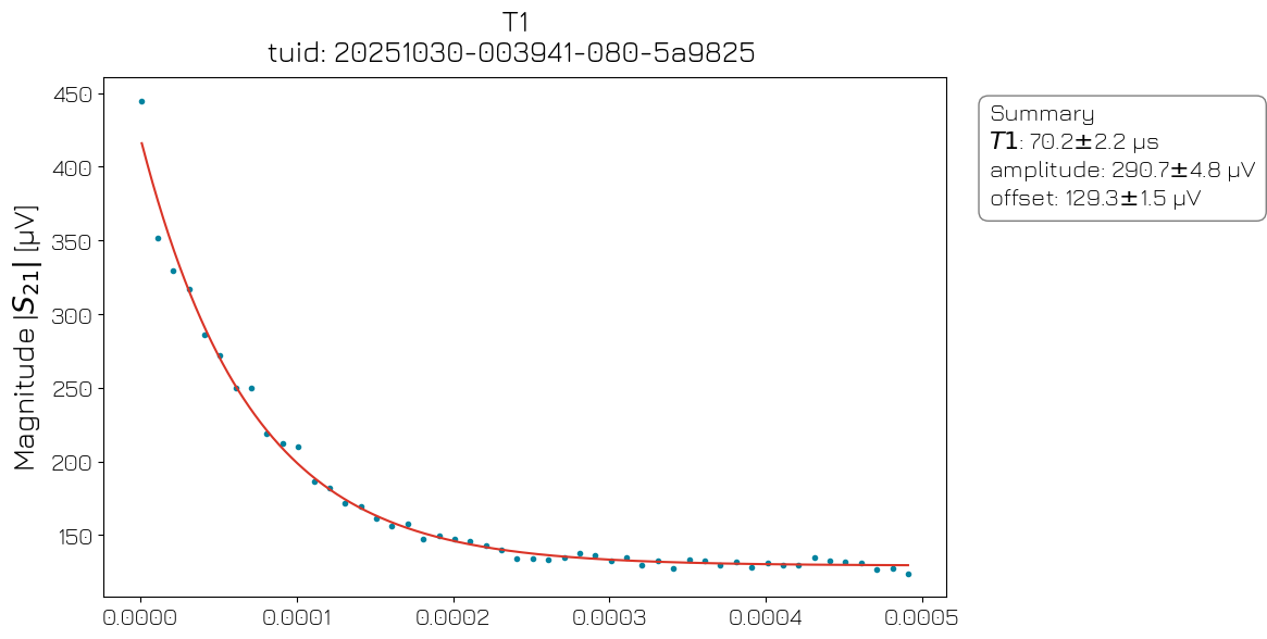
\(T_1\)

To analyze how quickly a qubit relaxes to the ground state from the excited state, a \(T_1\) experiment is performed. For this type of measurement, the qubit is initialized in the |0⟩ state and driven to the |1⟩ state using a π-pulse. By performing measurements at different times τ after the π-pulse the decay constant \(T_1\) can be measured.

Experiment settings

# Tau settings in seconds
tau_start = 1e-6  # s
tau_stop = 500e-6  # s
tau_step = 10e-6  # s

repetitions = 1000

Experiment schedule

t1_sched = Schedule(name="t1_experiment")

with (
    t1_sched.loop(arange(0, repetitions, 1, DType.NUMBER)),
    t1_sched.loop(arange(start=tau_start, stop=tau_stop, step=tau_step, dtype=DType.TIME)) as tau,
):
    t1_sched.add(Reset(qubit.name))
    # Prepare |1>
    t1_sched.add(X(qubit=qubit.name))
    # Measure after time tau
    t1_sched.add(Measure(qubit.name, coords={"tau": tau}, acq_channel="S_21"), rel_time=tau)

# Execute the experiment
t1_data = hw_agent.run(t1_sched)
if cluster.is_dummy:
    example_data = open_dataset("./dependencies/datasets/t1.hdf5", engine="h5netcdf")
    t1_data = t1_data.update({"S_21": example_data.S_21})

Analyze the experiment

t1_analysis = T1Analysis(t1_data).run()
t1_analysis.display_figs_mpl()

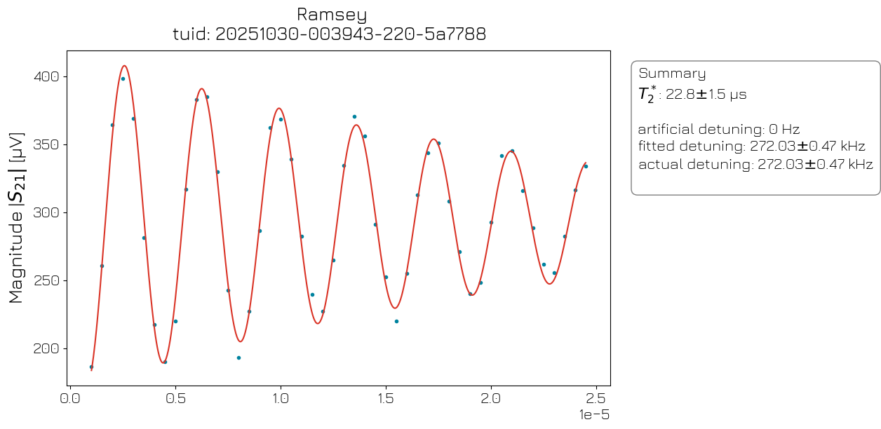
Ramsey

In a Ramsey experiment, the qubit is placed in a superposition of |0⟩ and |1⟩ using an \(X_{\pi/2}\) pulse, while a frequency offset is given to its port clock, such that the qubit accumulates a phase over time as it moves along the Bloch sphere equator. After some time τ, a second \(X_{\pi/2}\) pulse is played such that the qubit is moved either towards the |0⟩ or the |1⟩ state depending on its phase. By sweeping τ, an oscillation will be observed corresponding to the qubit’s detuning from its “true” \(f_{01}\) frequency, with a decay corresponding to the qubit’s \(T_2^*\).

Experiment settings

# Detuning
frequency_detuning = 1e6  # Hz

# Tau settings in seconds
tau_start = 1e-6  # s
tau_stop = 25e-6  # s
tau_step = 0.5e-6  # s

repetitions = 1000

Experiment schedule

Note: in order for the second \({\pi/2}\) pulse to have a phase difference \(\Delta \phi = \Delta f \tau\), relative to the first \(X_{\pi/2}\) pulse we offset the clock frequency by \(\Delta f\) for a time \(\tau\). Here, \(\Delta f\) is the frequency_detuning and \(\tau\) is tau.

ramsey_sched = Schedule(name="ramsey_experiment")
with (
    ramsey_sched.loop(arange(0, repetitions, 1, DType.NUMBER)),
    ramsey_sched.loop(
        arange(start=tau_start, stop=tau_stop, step=tau_step, dtype=DType.TIME)
    ) as tau,
):
    ramsey_sched.add(Reset(qubit.name))
    # Play X/2 pulse
    ramsey_sched.add(X90(qubit=qubit.name))

    # Implementing a phase kick:
    # Detune the qubit's clock by the required frequency detuning
    ramsey_sched.add(
        SetClockFrequency(
            clock=f"{qubit.name}.01",
            clock_freq_new=qubit.clock_freqs.f01 + frequency_detuning,
        )
    )
    # After a time tau, reset the qubit clock frequency to its original value
    ramsey_sched.add(
        SetClockFrequency(
            clock=f"{qubit.name}.01",
            clock_freq_new=qubit.clock_freqs.f01,
        ),
        rel_time=tau,
    )

    # Play second X/2 pulse after time tau
    ramsey_sched.add(X90(qubit=qubit.name))
    ramsey_sched.add(Measure(qubit.name, coords={"tau": tau}, acq_channel="S_21"))

# Execute the experiment
ramsey_data = hw_agent.run(ramsey_sched)
if cluster.is_dummy:
    example_data = open_dataset("./dependencies/datasets/ramsey.hdf5", engine="h5netcdf")
    ramsey_data = ramsey_data.update({"S_21": example_data.S_21})

Analyze the experiment

ramsey_analysis = RamseyAnalysis(ramsey_data).run()
ramsey_analysis.display_figs_mpl()

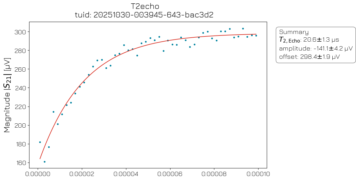
Echo

The Hahn echo experiment is a modified Ramsey sequence that uses a refocusing π-pulse at the midpoint of the free evolution time (t = τ/2) to invert the phase evolution, which effectively cancels out phase accumulations due to frequency offsets that are constant within the duration of the experiment (low-f noise). The fitted decay time \(T_{2,e}\) can be compared to \(T_2^*\) to estimate low-frequency noise.

Experiment settings

Note: in order for the second \({\pi/2}\) pulse to have a phase difference \(\Delta \phi = \Delta f \tau\), relative to the first \(X_{\pi/2}\) pulse we offset the clock frequency by \(\Delta f\) for a time \(\tau\). Here, \(\Delta f\) is the frequency_detuning and \(\tau\) is tau.

# Detuning
frequency_detuning = 1e6  # Hz

# Tau settings
tau_start = 1e-6  # s
tau_stop = 100e-6  # s
tau_step = 2e-6  # s

repetitions = 1000

Experiment schedule

echo_sched = Schedule(name="echo_experiment")
echo_sched.add(
    SetClockFrequency(
        clock=qubit.name + ".01", clock_freq_new=qubit.clock_freqs.f01 + frequency_detuning
    )
)
# Update parameters
echo_sched.add(IdlePulse(4e-9))

with (
    echo_sched.loop(arange(0, repetitions, 1, DType.NUMBER)),
    echo_sched.loop(arange(start=tau_start, stop=tau_stop, step=tau_step, dtype=DType.TIME)) as tau,
):
    echo_sched.add(Reset(qubit.name))
    # Play first X/2 pulse
    echo_sched.add(X90(qubit=qubit.name))
    # Add reflecting pi pulse at time tau / 2
    echo_sched.add(X(qubit=qubit.name), rel_time=tau / 2)
    # Play second X/2 pulse tau / 2 seconds after pi pulse
    echo_sched.add(X90(qubit=qubit.name), rel_time=tau / 2)
    echo_sched.add(Measure(qubit.name, coords={"tau": tau}, acq_channel="S_21"))

# Execute the experiment
echo_data = hw_agent.run(echo_sched)
if cluster.is_dummy:
    example_data = open_dataset("./dependencies/datasets/echo.hdf5", engine="h5netcdf")
    echo_data = echo_data.update({"S_21": example_data.S_21})

Analyze the experiment

echo_analysis = EchoAnalysis(echo_data).run()
echo_analysis.display_figs_mpl()

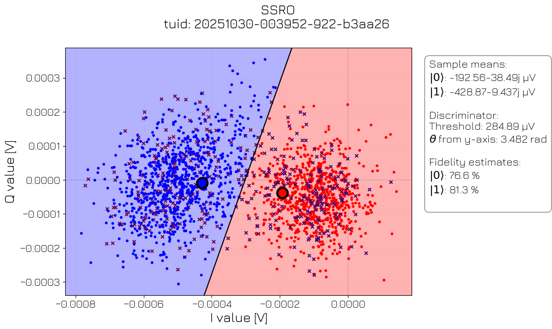
Single shot readout

This experiment is performed to calibrate single-shot readout for transmon qubits. The qubit is prepared in either the |0⟩ or |1⟩ state, after which the resonator response is plotted in the IQ plane. From the position of the two centroids a discriminator line is drawn that can be used on the FPGA to classify single shots of the readout resonator into the |0⟩ and |1⟩ qubit states. Furthermore, the structure of the two centroids allows us to quantify how well the two states can be distinguished and to find the State Preparation and Measurement (SPAM) errors. This experiment allows the user to determine the appropriate acquisition rotation and threshold, as described on the page documenting readout.

Experiment settings

num_shots = 1000

Experiment schedule

ssro_sched = Schedule("Readout")

with ssro_sched.loop(arange(start=0, stop=num_shots, step=1, dtype=DType.NUMBER)) as rep:
    ssro_sched.add(Reset(qubit.name))
    # Measure |0>
    ssro_sched.add(Measure(qubit.name, coords={"reps": rep, "state": 0}, acq_channel="S_21"))
    # Prepare |1>
    ssro_sched.add(Reset(qubit.name))
    ssro_sched.add(X(qubit=qubit.name))
    # Measure |1>
    ssro_sched.add(Measure(qubit.name, coords={"reps": rep, "state": 1}, acq_channel="S_21"))

# Execute the experiment
ssro_data = hw_agent.run(ssro_sched)
if cluster.is_dummy:
    example_data = open_dataset(
        "./dependencies/datasets/single_shot_readout.hdf5", engine="h5netcdf"
    )
    ssro_data = ssro_data.update({"S_21": example_data.S_21})

Analyze the experiment

ssro_analysis = SSROAnalysis(ssro_data).run()
ssro_analysis.display_figs_mpl()

Post-run

# Update device config
qubit.measure.acq_rotation = ssro_analysis.quantities_of_interest["acq_rotation_rad"].nominal_value
qubit.measure.acq_threshold = ssro_analysis.quantities_of_interest["acq_threshold"].nominal_value

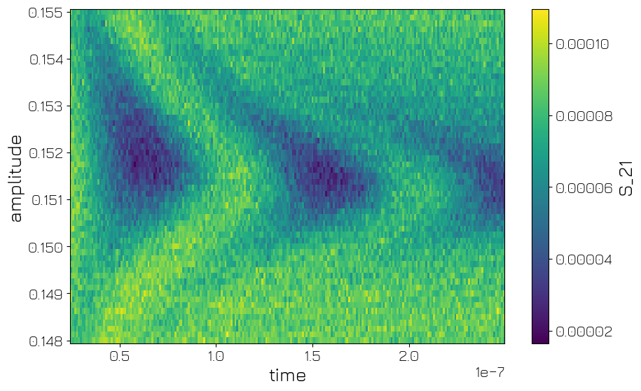
Coupled qubits characterization

This coupled-qubits characterization experiment aims to demonstrate two-qubit interactions between flux-tunable transmons. At the start of the experiment, two neighboring qubits with different \(f_{01}\) frequencies are prepared in the |1⟩ state. By playing a pulse on the flux line of the qubit with the highest frequency (\(q_0\) in this example), we can bring the |20⟩ and |11⟩ levels into resonance, which causes the two-qubit state to oscillate between the |11⟩ and |20⟩ states at a rate proportional to the coupling \(g\). For each full rotation \(\ket{11}\rightarrow\ket{20}\rightarrow\ket{11}\), the state picks up a global phase \(\pi\), which allows for the implementation of two-qubit gates. The goal of the characterization is to find the correct amplitude and duration of the pulse that should be played on the flux line of the high-frequency qubit, such that a \(\pi\) phase shift is accumulated, resulting in a CZ gate.

Experiment settings

# Flux settings
flux_start = 0.148
flux_stop = 0.155
flux_step = 0.000125

# Time settings
time_start = 25e-9
time_stop = 250e-9
time_step = 1e-9

repetitions = 1

Experiment schedule

coupled_qubits_sched = Schedule("coupled_qubits")

with (
    coupled_qubits_sched.loop(arange(0, repetitions, 1, DType.NUMBER)),
    coupled_qubits_sched.loop(arange(flux_start, flux_stop, flux_step, DType.AMPLITUDE)) as amp,
    coupled_qubits_sched.loop(arange(time_start, time_stop, time_step, DType.TIME)) as time,
):
    # Prepare both qubits in |0>
    start = coupled_qubits_sched.add(Reset(q0.name, q2.name))

    # Prepare both qubits in |1>
    coupled_qubits_sched.add(X(q0.name), ref_op=start)
    coupled_qubits_sched.add(X(q2.name), ref_op=start)

    # Play square pulse over the flux line of q0
    flux_pulse = coupled_qubits_sched.add(SquarePulse(amp=amp, duration=time, port=f"{q0.name}:fl"))

    # Measure q0
    coupled_qubits_sched.add(
        Measure(q0.name, coords={"amplitude": amp, "time": time}, acq_channel="S_21"),
        ref_op=flux_pulse,
    )

# Execute the experiment
coupled_qubits_data = hw_agent.run(coupled_qubits_sched)
if cluster.is_dummy:
    example_data = open_dataset("./dependencies/datasets/cphase_chevrons.hdf5", engine="h5netcdf")
    coupled_qubits_data.update({"S_21": example_data.S_21})

Analyze the experiment

coupled_qubits_data = acq_coords_to_dims(coupled_qubits_data, ["amplitude", "time"], "S_21")
np.abs(coupled_qubits_data.S_21).plot()

<matplotlib.collections.QuadMesh at 0x7f0236be0760>

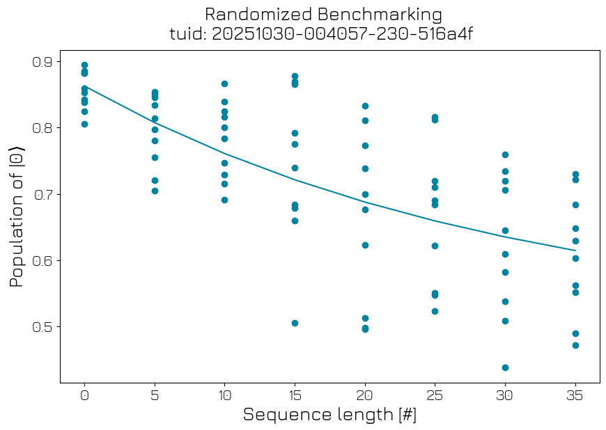
Single qubit randomized benchmarking

Single-qubit randomized benchmarking measures the single-qubit gates fidelity. For this experiment a sequence of random Clifford gates is generated (one sequence per seed), and for each experiment an increasing portion of this sequence is executed (different gate string lengths m) before the qubit is returned to its initial state. A fit of the exponential decay of the overlap between initial and final states gives the average error per Clifford gate, while the variance in this \(⟨\psi_f|\psi_i⟩\) overlap between seeds for the same gate string length gives an estimate of the degree to which this error is coherent.

Experiment settings

# RB settings
lengths = np.arange(0, 40, 5)
seeds = np.random.randint(0, 2**31 - 1, size=10, dtype=np.int32)

repetitions = 1

Experiment schedule

sched = randomized_benchmarking_schedule(
    qubit.name,
    lengths=lengths,
    repetitions=repetitions,
    seeds=seeds,
)

# Execute the experiment
rb_data = hw_agent.run(sched)
if cluster.is_dummy:
    example_data = open_dataset(
        "./dependencies/datasets/single_qubit_randomized_benchmarking.hdf5", engine="h5netcdf"
    )
    rb_data.update({"S_21": example_data.S_21, "calibration": example_data.calibration})

Analyze the experiment

rb_analysis = RBAnalysis(rb_data).run()
rb_analysis.display_figs_mpl()

/builds/0/.venv/lib/python3.10/site-packages/numpy/lib/_function_base_impl.py:644: ComplexWarning: Casting complex values to real discards the imaginary part
  a = asarray(a, dtype=dtype, order=order)
/builds/0/.venv/lib/python3.10/site-packages/matplotlib/cbook.py:1719: ComplexWarning: Casting complex values to real discards the imaginary part
  return math.isfinite(val)
/builds/0/.venv/lib/python3.10/site-packages/matplotlib/collections.py:200: ComplexWarning: Casting complex values to real discards the imaginary part
  offsets = np.asanyarray(offsets, float)

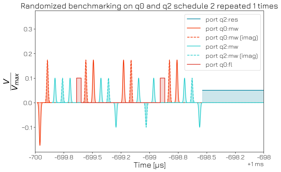
Two-qubit randomized benchmarking

Two-qubit randomized benchmarking characterizes the overall Clifford (in)fidelity, which includes contributions from both single- and two-qubit gates. For this experiment a random sequence of two-qubit Cliffords is generated (one sequence per seed), and for each experiment an increasing portion of this sequence is executed (different gate string lengths \(m\)) before the two qubits are returned to their initial states. A fit of the exponential decay of the overlap between initial and final states gives the average error per gate, while the variance in this \(⟨\psi_f|\psi_i⟩\) overlap between seeds for the same gate string length gives an estimate of the degree to which this error is coherent.

Experiment settings

# RB settings
lengths = [1]  # number
seeds = np.random.randint(0, 2**31 - 1, size=1, dtype=np.int32)  # number
repetitions = 1

Experiment schedule

sched = randomized_benchmarking_schedule(
    [q0.name, q2.name],
    lengths=lengths,
    repetitions=repetitions,
    seeds=seeds,
    generator=TwoQubitCliffordCZ,  # Change to the appropriate gate for your architecture!
)

# Compile the schedule
comp_sched = hw_agent.compile(sched)

Show the schedule

fig, ax = comp_sched.plot_pulse_diagram(plot_backend="mpl")
ax.set_xlim(q2.reset.duration, q2.reset.duration + 2e-6)
plt.show()

Update the device configuration file

After measurement, we may store the measured device properties inside a new file to use in future experiments. The time-unique identifier ensures that it is easy to find back previously found measurement results.

hw_agent.quantum_device.to_json_file("./dependencies/configs", add_timestamp=True)

'./dependencies/configs/two_flux_tunable_transmons_2025-10-30_00-40-57_UTC.json'