Qblox Scheduler - Pulse level tutorial 0#

In this tutorial, we will continue from the Qblox Scheduler - Hello World tutorial!. Previously, a the Qblox Scheduler program was created and executed with the HardwareAgent without any added content in our schedule. Now we will expand our schedule by defining pulses on each module and output them from the hardware. The tutorial will be utilizing all the existing modules in the Qblox Cluster series, however each module in the tutorial can be run independently to execute pulses on the desired modules.

As done in the Qblox Scheduler - Hello World!, we need to define the hardware which will be used for this tutorial, via the hardware configuration file. The hardware configuration file which is to be used can be seen here and is defined on the following path:

[1]:

hardware_cfg = "dependencies/hardware.json"

As previously done, we allow the communicator of HardwareAgent get to know our hardware by passing on the hardware configuration file inside the hardware agent as an argument

[2]:

from qblox_scheduler import HardwareAgent

agent = HardwareAgent(hardware_cfg)

QCM#

We will start with executing pulses on the QCM and go from there.

The QCM is a baseband module (0 - 400 MHz) with 4 channel outputs. In this section, we will utilize this functionality to output a modulated pulse with a certain frequency on one of its outputs.

First we need to define our schedule which will later include our pulse and the frequency in which we modulate our signal:

[3]:

from qblox_scheduler import Schedule

qcm_schedule = Schedule("QCM pulse schedule")

Note: Since we are introducing each concept one by one to clarify each component to build your Qblox Scheduler program on the pulse level, the import of certain functions happens at each code instance where necessary. In general, all imports can be included at the beginning of the program.

Now we can add our desired pulses in the created schedule.

[4]:

from qblox_scheduler import ClockResource
from qblox_scheduler.operations import SquarePulse

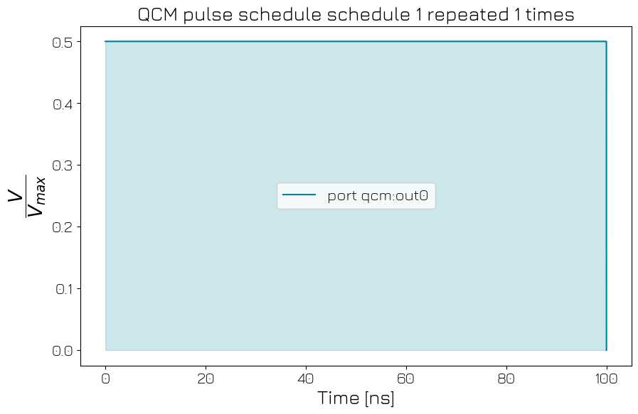
qcm_schedule.add(SquarePulse(amp=0.5, duration=100e-9, port="qcm:out0", clock="qcm.out0"))
qcm_schedule.add_resource(ClockResource(name="qcm.out0", freq=100e6))

The schedule above will execute a square pulse, modulated with a frequency of 100 MHz (indicated by the clock) and will be outputted on the port connected to O1 on the QCM (as the square pulse specifies port out0 and in the hardware configuration file, port qcm:out0 is connected to output 1 of the module in slot 2 which is where our QCM is situated).

Note: Ensure that the port name matches the port name associated with the desired module in the connectivity of the hardware configuration file. This is how Qblox Scheduler is able to connect a certain pulse in a schedule with the modules housed inside the Cluster.

To execute the schedule, we pass our schedule as an argument to the HardwareAgent.

[5]:

agent.run(qcm_schedule)

/builds/0/.venv/lib/python3.10/site-packages/qblox_scheduler/qblox/hardware_agent.py:460: UserWarning: cluster0: Trying to instantiate cluster with ip 'None'.Creating a dummy cluster.
  warnings.warn(

[5]:

<xarray.Dataset> Size: 0B
Dimensions:  ()
Data variables:
    *empty*
Attributes:
    tuid:     20251118-154430-710-485ce2

In order to check the pulse diagram of our created schedule, we can utilize the plot_pulse_diagram which creates a visualization of the pulses defined in the schedule above.

[6]:

compiled_qcm_schedule = agent.compile(qcm_schedule)
compiled_qcm_schedule.plot_pulse_diagram()

[6]:

(<Figure size 1000x621 with 1 Axes>,
 <Axes: title={'center': 'QCM pulse schedule schedule 1 repeated 1 times'}, xlabel='Time [ns]', ylabel='$\\dfrac{V}{V_{max}}$'>)

../../../_images/applications_setupguides_any_setupqbloxscheduler_11_1.png

Note: There are numerous pulses which can be executed with Qblox Scheduler. The pulses which are available can be found in the pulse library API.

QCM-RF#

The RF modules contain onboard LO and IQ mixers, which allows to output signals between 2-18.5 GHz, in contrast to the baseband modules. The QCM-RF has two physical output ports and here we will utilize one of the outputs to create a schedule on the pulse level, which outputs a signal in the mentioned frequency range with Qblox Scheduler.

[9]:

qcm_rf_schedule = Schedule("QCM-RF pulse schedule")

qcm_rf_schedule.add(SquarePulse(amp=0.9, duration=1e-6, port="qcm_rf:out0", clock="qcm_rf.out0"))
qcm_rf_schedule.add_resource(ClockResource(name="qcm_rf.out0", freq=4.5e9))

The schedule will output a modulated square pulse of 4.5 GHz on output O1 of the QCM-RF.

To execute the schedule we pass our schedule as an argument to the HardwareAgent.

[10]:

agent.run(qcm_rf_schedule)

[10]:

<xarray.Dataset> Size: 0B
Dimensions:  ()
Data variables:
    *empty*
Attributes:
    tuid:     20251118-154431-690-dff5ba

QTM#

The QTM is the timetagging module and used for photon counting. With its 8 SMP channels, each channel can be configured to act as inputs or outputs.

[13]:

from qblox_scheduler.operations import IdlePulse, MarkerPulse

qtm_schedule = Schedule("QTM pulse schedule")

qtm_schedule.add(MarkerPulse(duration=100e-9, port="qtm:out0"))
qtm_schedule.add(IdlePulse(duration=4e-9))

[13]:

{'name': 'c7491a76-ea83-40a7-8c24-ad4a9c4b0d0b', 'operation_id': '-4309106413334689536', 'timing_constraints': [TimingConstraint(ref_schedulable=None, ref_pt=None, ref_pt_new=None, rel_time=0)], 'label': 'c7491a76-ea83-40a7-8c24-ad4a9c4b0d0b'}

Note: Since there is a marker pulse which is set, it requires at least 4 ns for it to be executed. Therefore we need to add an idling pulse to activate the marker pulse.

With the QTM executing trigger pulses, the pulse which can be executed as an output pulse from the QTM is the MarkerPulse. This pulse is executed on the port qtm0:out which is connected to the channel 1 on the QTM.

[14]:

agent.run(qtm_schedule)

[14]:

<xarray.Dataset> Size: 0B
Dimensions:  ()
Data variables:
    *empty*
Attributes:
    tuid:     20251118-154432-054-0cd10a

Qblox Scheduler - Pulse level tutorial 0#

QCM#

QRM#

QCM-RF#

QRM-RF#

QTM#