Qblox Instruments Tutorial 0#

This tutorial is meant as a sequel to the Qblox Instruments Hello World Tutorial.

The objective of this tutorial is to familiarize you with the basic control and operation of our modules using the Qblox Instruments driver.

Standard Imports#

[1]:

from __future__ import annotations

import matplotlib.pyplot as plt
import numpy as np
import rich
import scipy.signal
from IPython.lib.pretty import pprint

## QCoDeS helper function
from qcodes.instrument import find_or_create_instrument

## Driver for Qblox Instruments
from qblox_instruments import Cluster, ClusterType

Connecting to the cluster#

[2]:

cluster_ip = "10.10.200.42"
cluster_name = "cluster0"

[3]:

## Helper function from QCoDeS, imported above.
cluster: Cluster = find_or_create_instrument(
    Cluster,
    recreate=True,
    name=cluster_name,
    identifier=cluster_ip,
    ## If you keep cluster ip as None, then you can "connect" to a dummy instrument.
    ## This can be used to check your code without connecting to an actual cluster.
    dummy_cfg=(
        {
            2: ClusterType.CLUSTER_QCM,
            4: ClusterType.CLUSTER_QRM,
            6: ClusterType.CLUSTER_QCM_RF,
            8: ClusterType.CLUSTER_QRM_RF,
            10: ClusterType.CLUSTER_QTM,
            12: ClusterType.CLUSTER_QRC,
        }
        if cluster_ip is None
        else None
    ),
    debug=False,
)

### If you do NOT wish to use QCoDeS, you can also run the following line. However, note that if a Cluster object with the same name already exists, it will throw a KeyError: Instrument with name <cluster_name> already exists.
# cluster: Cluster = Cluster(name = cluster_name, identifier=cluster_ip)

/.venv/lib/python3.14/site-packages/qblox_instruments/qcodes_drivers/cluster.py:70: FutureWarning: Passing a boolean argument for the `debug` parameter is deprecated and could cause unexpected behaviour in a future version.
  warnings.warn(

Resetting the cluster#

[4]:

cluster.reset()
print(cluster.get_system_status())

Status: ERROR, Flags: FEEDBACK_NETWORK_CALIBRATION_FAILED, Slot flags: SLOT2_FEEDBACK_NETWORK_CALIBRATION_FAILED, SLOT4_FEEDBACK_NETWORK_CALIBRATION_FAILED, SLOT6_FEEDBACK_NETWORK_CALIBRATION_FAILED, SLOT8_FEEDBACK_NETWORK_CALIBRATION_FAILED, SLOT10_FEEDBACK_NETWORK_CALIBRATION_FAILED, SLOT12_FEEDBACK_NETWORK_CALIBRATION_FAILED

Getting the relevant modules#

[5]:

# This helper function fetches back the modules available in the cluster. The argument of this function can be used to filter by module type. See the commented examples below.
modules = cluster.get_connected_modules()

## For fetching all QCMs
qcms = cluster.get_connected_modules(lambda mod: mod.is_qcm_type and not mod.is_rf_type)
print("QCMs:", qcms)

## For fetching all QRMs
qrms = cluster.get_connected_modules(lambda mod: mod.is_qrm_type and not mod.is_rf_type)
print("QRMs:", qrms)

## For fetching all QCM-RFs
qcm_rfs = cluster.get_connected_modules(lambda mod: mod.is_qcm_type and mod.is_rf_type)
print("QCM-RFs:", qcm_rfs)

## For fetching all QRM-RFs
qrm_rfs = cluster.get_connected_modules(lambda mod: mod.is_qrm_type and mod.is_rf_type)
print("QRM-RFs:", qrm_rfs)

## For fetching all QTMs
qtms = cluster.get_connected_modules(lambda mod: mod.is_qtm_type)
print("QTMs:", qtms)


## Seeing the dictionary with all the fetched modules
modules

QCMs: {2: <QCM, cluster0_module2>}
QRMs: {4: <QRM, cluster0_module4>}
QCM-RFs: {6: <QCM-RF, cluster0_module6>}
QRM-RFs: {8: <QRM-RF, cluster0_module8>}
QTMs: {10: <QTM, cluster0_module10>}

[5]:

{2: <QCM, cluster0_module2>,
 4: <QRM, cluster0_module4>,
 6: <QCM-RF, cluster0_module6>,
 8: <QRM-RF, cluster0_module8>,
 10: <QTM, cluster0_module10>,
 12: <QRC, cluster0_module12>}

Selecting the modules#

Please comment the modules that are not present in your cluster! You can skip the corresponding sections ahead as well.

Note that identical modules are identified by an incrementing index, with 0 being the leftmost module in the cluster.

[6]:

qcm = list(qcms.values())[0] if qcms else None
qrm = list(qrms.values())[0] if qrms else None
qcm_rf = list(qcm_rfs.values())[0] if qcm_rfs else None
qrm_rf = list(qrm_rfs.values())[0] if qrm_rfs else None
qtm = list(qtms.values())[0] if qtms else None

Setup#

Before we proceed, we specify the connections between the modules and to the oscilloscope.

QCM:
- Output 1 (O1) to oscilloscope channel 2.
- Marker channel 1 (marker corresponding to O1) to oscilloscope channel 1.
- Output 2 (O2) to QRM input 2 (I2).
QRM:
- Output 1 (O1) to oscilloscope channel 3.
- Output 2 (O2) to QRM input 1 (I1).
QCM-RF:
- Output 1 (O1) to oscilloscope channel 4.
QRM-RF:
- Output 1 (O1) to Input 1(I1)
Oscilloscope:
- Channel 1 to QCM marker 1. This channel is set as the trigger for the scope. Trigger set to rising edge, trigger level ~700mv.
- Channel 2 to QCM O1
- Channel 3 to QRM O1
- Channel 4 to QCM-RF O1
- Vertical scale for all channels can be set to around 1 V/division
- Horizontal timebase can be set to around 40 ns/division

Now you are ready to execute some experiments! Please note that the sections are divided according to module type, and they are designed to work together if you have one of each module. In the event that you only have a selection of such modules, you can execute just those parts but it’s still advised to read through the sections for the baseband modules (titled “Only QCM” and “QCM and QRM”) to understand the general flow.

Only QCM#

We begin this exercise by generating an un-modulated Gaussian pulse from the QCM O1 using waveform memory. We will not use the Digital/Numerically Controlled Oscillator (NCO) here.

Let us first study the wave generation/AWG path of the QCM. Please refer to the image below.

To learn in more detail about the sequencers present in Qblox modules, please see the Cluster Sequencer pages.

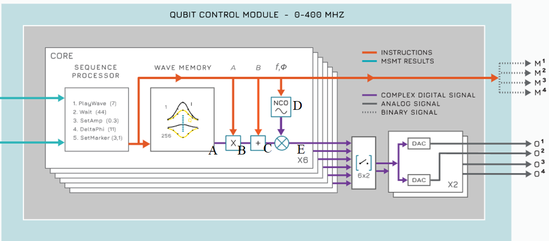
Let’s follow this diagram using equations. We use the standard convention of denoting signals with complex numbers here. The real part of the signal (at all stages A-E) tells us what is going on in path 0 of the sequencer (also known as the I path for “in-phase”), while the imaginary part is the signal generated in path 1 of the sequencer (also known as the Q path for “quadrature”).

Output of the waveform memory (A): As mentioned in the previous tutorial, the waveform memory stores the envelopes we are interested in using. The waveforms are accessed via the play x, y, duration instruction, which plays the envelopes at indices x and y on AWG path 0 and path 1 (or the I and Q paths) respectively, for a minimum of duration nanoseconds.

Let us denote the signal at A as

\[a(t) + j \cdot b(t),\]

where $a(t), b(t)$ refer to the envelopes being played, and $j = \sqrt{-1}$.
Parameterization through the AWG gain (B): The gain for both AWG paths can be set independently via the Q1ASM command (for dynamic parameterization) set_awg_gain or (for static parameterization) via the API instructions Sequencer.gain_awg_path0(), Sequencer.gain_awg_path1(). See the Q1ASM instructions page and the Sequencer API reference for more details on setting the gain via Q1ASM and the API respectively.

Therefore, the signal at B is

\[A(t) + j \cdot B(t),\]

where $A(t) = total\_path\_0\_gain * a(t)$, $B(t) = total\_path\_1\_gain * b(t)$ and $total\_gain = static\_gain * dynamic\_gain$. For this simple example we will not be using any gains.
Parameterization through the AWG offset (C): Independent offsets can be set for AWG path 0 and path 1, denoted by the single complex number $o$ here. This can be done via Q1ASM (for dynamic parameterization) through the instruction set_awg_offs or (for static parameterization) via the API instructions Sequencer.offset_awg_path0(), Sequencer.offset_awg_path1(). See the Q1ASM instructions page and the Sequencer API reference for more details on setting the AWG offset via Q1ASM and the API respectively.

Therefore, the signal at C is

\[A(t) + j \cdot B(t) + o,\]

where $o \in \mathbb C = static\_offset + dynamic\_offset$.
Parameterization through the Numerically Controlled Oscillator (NCO) (D): Each sequencer in our modules has an independent digital oscillator called the NCO. The NCO is under the absolute control of the user, allowing complete control of the frequency and phase at every point in time.

We will represent the output signal provided by the NCO (that is, the signal at D) as

\[e^{j(2\pi ft + \phi)}\]

where $f$ is the set NCO frequency, and $\phi$ is the phase. Note that this implies that the NCO provides signals in quadrature to the IQ mixer for multiplication with the signal C . If you are not familiar with I/Q signals, we recommend you to refer to this article.

The frequency of the of the NCO can be set dynamically via the set_freq Q1ASM instruction, or statically via the API instruction Sequencer.nco_freq(). Note that one must never try to control the NCO via both static and dynamic parameterization. This will lead to undefined behavior due to a race condition between static and dynamic NCO frequency.

The phase of the NCO can be set dynamically via the set_ph or set_ph_delta Q1ASM instructions, or statically via the API instruction Sequencer.nco_phase_offs(). Again, note that one must never try to control the NCO via both static and dynamic parameterization. This will lead to undefined behavior due to a similar race condition between the static and dynamic phase offsets.

For more details about the NCO please see the NCO tutorial and the Cluster Sequencer pages.
Final Sequencer Output after IQ mixing (E): The last step before the sequencer output, as seen from the block diagram above, is the digital IQ mixing of the signals C and D. IQ mixing corresponds to simply multiplying the complex signals at the input of the IQ mixer. Note that the mixing of the NCO signal into the AWG path can be turned on or off by using the API instruction Sequencer.mod_en_awg(True/False) respectively.

Therefore the signal at E is

\[(A(t) + j \cdot B(t) + o) \cdot e^{j(2\pi ft + \phi)}\]

\[= A(t)\cdot e^{j(2\pi ft + \phi)} + j \cdot B(t)\cdot e^{j(2\pi ft + \phi)} + o\cdot e^{j(2\pi ft + \phi)}.\]

\[= A(t)\cdot e^{j(2\pi ft + \phi)} + B(t)\cdot e^{j \frac{\pi}{2}} \cdot e^{j(2\pi ft + \phi)} + o\cdot e^{j(2\pi ft + \phi)}.\]

Let us interpret this final output signal:
- The first term corresponds to a simple upconversion of the (rescaled) envelope played on path 0 by the NCO frequency
- The second term corresponds to an upconversion of the (rescaled) envelope played on path 1 by the NCO frequency, phase shifted by $90^\circ$.
- The third and last term corresponds simply to the modulation of a constant offset by the NCO; that is, a CW tone with amplitude $=|o|$, frequency $=f$ and phase $=\angle o + \phi$!

Using this information, we will now generate an unmodulated Gaussian from the QCM O1.

Looking at the equations above, we can use the strategy:

$A(t) = $ Gaussian envelope.
$B(t) = $ arbitrary.
Not setting an NCO frequency or phase, so $f = 0, \phi = 0$
No offset or gain on any path, so $o = 0$ and $A(t) = a(t), B(t) = b(t)$

Taking all this into account, the final sequencer output should be

\[A(t)\cdot e^{j(2\pi (0)t + (0))} + B(t)\cdot e^{j \frac{\pi}{2}} \cdot e^{j(2\pi (0)t + (0))} + (0)\cdot e^{j(2\pi (0)t + (0))}\]

\[= a(t) + j \cdot b(t).\]

Hence, if we map the real output the sequencer (the I path/AWG path 0) - to O1, we should see the signal $a(t)$ on the scope.

Creating the `waveforms` dictionary#

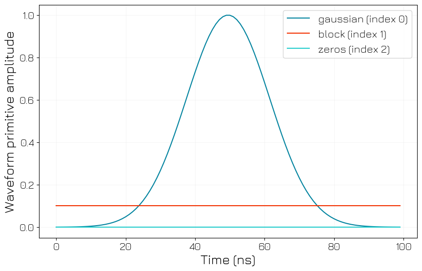
Let’s upload the waveforms that we want to output.

[7]:

# Waveform parameters
waveform_length = 100  # nanoseconds

# Waveform dictionary (data will hold the samples and index will be used to select the waveforms in the instrument).
waveforms = {
    "gaussian": {
        "data": scipy.signal.windows.gaussian(waveform_length, std=0.12 * waveform_length).tolist(),
        "index": 0,
    },
    "block": {"data": [0.1 for i in range(0, waveform_length)], "index": 1},
    "zeros": {"data": [0.0 for i in range(0, waveform_length)], "index": 2},
}

Let’s plot the waveforms to see what we have created.

[8]:

time = np.arange(0, max(len(d["data"]) for d in waveforms.values()), 1)
fig, ax = plt.subplots(1, 1)

for wf, d in waveforms.items():
    ax.plot(time[: len(d["data"])], d["data"], label=str(wf) + " (index " + str(d["index"]) + ")")

ax.legend()
ax.grid(alpha=1 / 10)
ax.set_ylabel("Waveform primitive amplitude")
ax.set_xlabel("Time (ns)")

plt.draw()
plt.show()

../../../_images/applications_setupguides_any_setupqbloxinstruments_20_0.png

Writing our Q1ASM sequence program#

Let us now write our Q1ASM sequence program.

[9]:

qcm_seq_prog = """

    ## Synchronize all sequencers
    wait_sync 4

    ## Setting marker output 1 to high. The argument of the set_mrk instruction works like a mask - simply convert the argument
    ## to a 4 bit binary number, and the marker channels corresponding to the bits that are set will be set to high.

    set_mrk 1  # 0b0001
    ## In this case, we choose the binary number 0001, so marker channel 1 will be set to high and all others will remain at 0.

    ## Play the waveforms stored at index 0 (the Gaussian) and index 1 (the block) and wait 4 ns.

    stop

"""

Note that:

The marker and channel outputs have the same path length, so they will appear simultaneously on the scope.
For more details on the play and set_mrk instructions, see the Q1ASM instructions page
The effect of wait_sync becomes apparent when using more than one sequencer, as seen in the next section.

Creating and Uploading the sequence dictionary#

Since we have defined our waveforms and Q1ASM sequence program, let’s construct and upload the sequence dictionary.

[10]:

# Add sequence to single dictionary
qcm_sequence = {
    "waveforms": waveforms,
    "weights": {},
    "acquisitions": {},
    "program": qcm_seq_prog,
}

# Upload sequence.
qcm.sequencer0.sequence(qcm_sequence)

Configuring QCoDeS (static and analog) parameters#

Adding the sequencer to the SYNQ network#

[11]:

# Configure the sequencer to synchronize.
qcm.sequencer0.sync_en(True)

Channel Map#

We now map the sequencer outputs to the physical module outputs.

[12]:

# Map the sequencer to specific outputs (but first disable all sequencer connections).
qcm.disconnect_outputs()

# We will map the I channel / path 0 to output 0 (O1) and the Q channel / path 1 to output 1 (O2)
qcm.sequencer0.connect_out0("I")
qcm.sequencer0.connect_out1("Q")

Arming and starting the sequencer#

Finally, we arm and start the sequencers.

[13]:

# Arm and start the sequencer.
qcm.arm_sequencer(0)

qcm.start_sequencer()

# Print status of both sequencers.
print(qcm.get_sequencer_status(0))

Status: OKAY, State: STOPPED, Info Flags: NONE, Warning Flags: NONE, Error Flags: NONE, Log: []

Oscilloscope Output#

As expected, we see the simultaneous outputs from channels 1 and 2; that is, the marker channel goes high (3.3V TTL) and the QCM O1 generates an unmodulated Gaussian.

QCM and QRM#

NB: Please SKIP this section if you do not have a QRM or QRM-RF.

Let’s now use two modules simultaneously.

We will

Output an unmodulated Gaussian from the QCM and QRM O1.
Output an unmodulated square/block pulse from QCM O2, which is connected to QRM I2.
Output an unmodulated square/block pulse from QRM O2, which is connected to QRM I1.
Read-in the input signals from QRM I1 and I2 and
1. Study the acquired data, including both “scope” and “bin” data structures
2. Plot the returned “scope” data
3. Analyze the integrated “bin” values

We will re-use the waveform dictionary from above, so let’s begin writing the Q1ASM program.

Define waveforms#

[14]:

# Waveform parameters
waveform_length = 100  # nanoseconds

# Waveform dictionary (data will hold the samples and index will be used to select the waveforms in the instrument).
waveforms = {
    "gaussian": {
        "data": scipy.signal.windows.gaussian(waveform_length, std=0.12 * waveform_length).tolist(),
        "index": 0,
    },
    "block": {"data": [0.1 for i in range(0, waveform_length)], "index": 1},
    "zeros": {"data": [0.0 for i in range(0, waveform_length)], "index": 2},
}

Q1ASM program#

[15]:

qrm_seq_prog = """

    ## We use this instruction (along with the sync_en instruction) to synchronize the QCM and QRM sequencer
    wait_sync 4
    ## After this point, we can assume that the QCM and QRM sequencers share a common time axis.

    ## Playing Gaussian (index 0) on I channel and Block (index 1) on Q channel
    play 0,1,4

    ## Acquiring the signal from the I and Q acquisition paths. Note that this will not interrupt the play
    ## We acquire into the acquisition dictionary at index 0 and store the integrated value in bin 0
    acquire 0,0,4

    stop

"""

For more details about the acquire instruction please see the Q1ASM instructions page.

Creating the acquisition dictionary#

We must specify the index of the acquisition and the number of bins we wish to use.

[16]:

# Acquisitions
qrm_acquisitions = {
    "single": {"num_bins": 1, "index": 0},
}

Creating and uploading the sequence dictionary#

Now that we have defined our waveforms, acquisitions, and sequence program, we can construct and upload our sequencer dictionary.

[17]:

# Add sequence to single dictionary
qrm_sequence = {
    "waveforms": waveforms,
    "weights": {},
    "acquisitions": qrm_acquisitions,
    "program": qrm_seq_prog,
}

# Upload sequence.
qrm.sequencer0.sequence(qrm_sequence)

Configuring QCoDeS parameters via API#

Adding the sequencer to the SYNQ network#

Recall that unless the cluster is reset, the set parameters remain in the modules. Hence, we do not need to add the QCM sequencer 0 the SYNQ network here.

[18]:

# Configure the sequencers to synchronize.
# Note that we can simply add the QRM sequencer since the QCM sequencer was already added.
if qrms:
    qrm.sequencer0.sync_en(True)

Channel map#

We only need to create a channel mapping for QRM sequencer 0 since the QCM channel map was created earlier and will be preserved.

[19]:

# Map sequencers to specific outputs (but first disable all sequencer connections).
qrm.disconnect_outputs()
qrm.disconnect_inputs()

# Connect sequencer 0 I and Q to O1 and O2 respectively
qrm.sequencer0.connect_out0("I")
qrm.sequencer0.connect_out1("Q")

# Connect sequencer 0 acquisition channel I and Q to I1 and I2 respectively
qrm.sequencer0.connect_acq_I("in0")
qrm.sequencer0.connect_acq_Q("in1")

We need to configure a few more settings to enable scope data storage.

[20]:

# Configure scope mode
# Here we tell the module that sequencer 0 will trigger the scope acquisition.
# We also specify that the scope acquisitions for path 0 and path 1 will be triggered
# in the sequence program via the acquire instruction.

qrm.scope_acq_sequencer_select(0)
qrm.scope_acq_trigger_mode_path0("sequencer")
qrm.scope_acq_trigger_mode_path1("sequencer")


# Configure integration.
# We tell the module to integrate the first 1000 scope values to store in the bin.
qrm.sequencer0.integration_length_acq(1000)

As previously mentioned, the uploaded sequence and QCoDeS settings persist on the module unless the cluster is reset.

Hence, we can simply arm and start the QCM again to see the same result as before.

Note that all relevant modules must be armed first and then started.

Arming and starting the sequencers#

[21]:

# Arm and start both sequencers.
if qcms:
    qcm.arm_sequencer(0)

qrm.arm_sequencer(0)

cluster.start_sequencer()

# Print status of both sequencers.
print(qcm.get_sequencer_status(0))
print(qrm.get_sequencer_status(0))

Status: OKAY, State: STOPPED, Info Flags: NONE, Warning Flags: NONE, Error Flags: NONE, Log: []
Status: OKAY, State: STOPPED, Info Flags: ACQ_SCOPE_DONE_PATH_0, ACQ_SCOPE_DONE_PATH_1, ACQ_BINNING_DONE, Warning Flags: NONE, Error Flags: NONE, Log: []

Oscilloscope Output#

QCM_and_QRM_scope_output

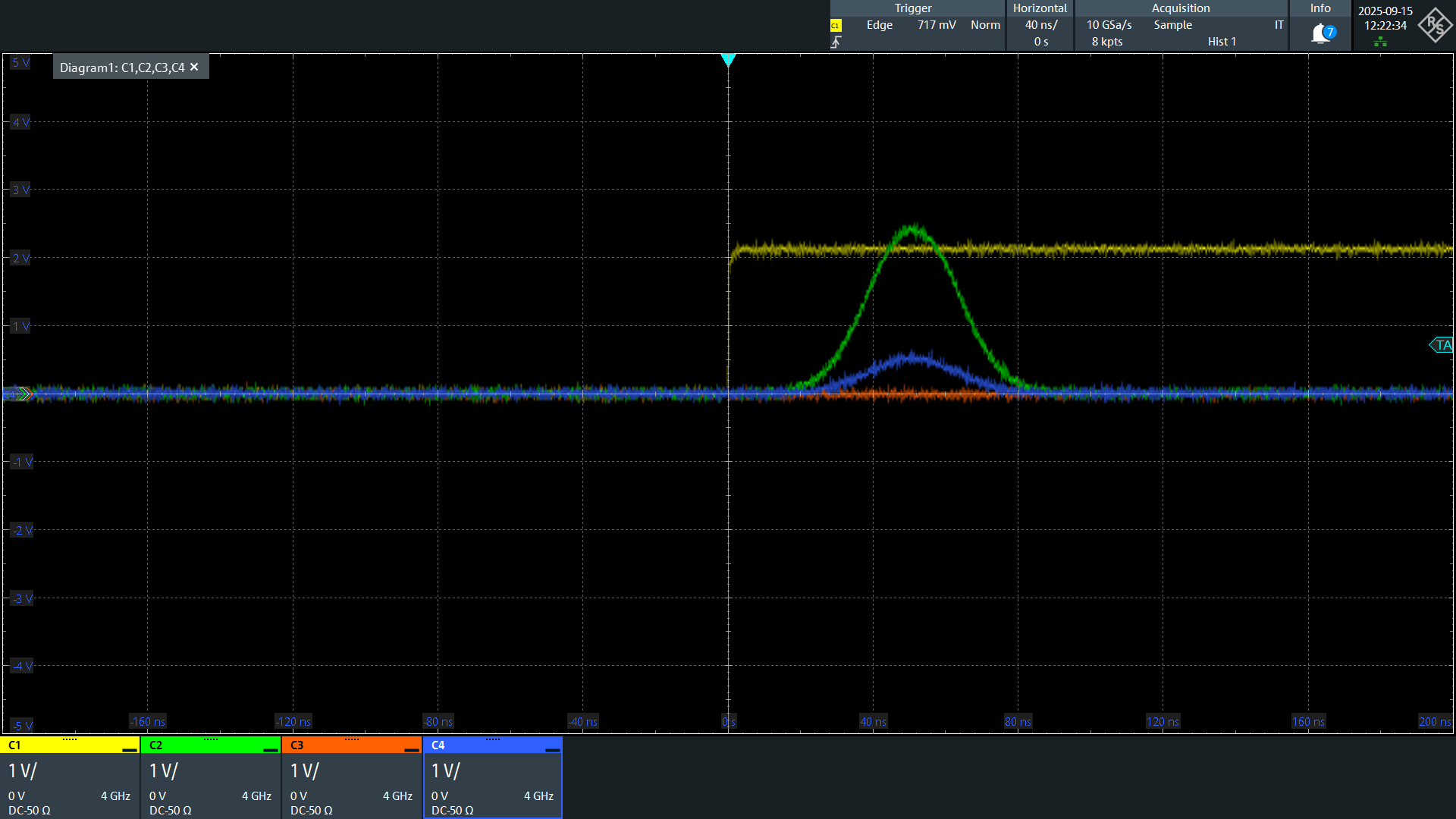
Once again, we see the expected output from both modules.

Fetching the acquisition data from the QRM#

[22]:

# Before fetching let us see if the acquisition has finished
qrm.sequencer0.get_acquisition_status(timeout=1)

[22]:

True

Now we will tell the QRM to store the scope data in the acquisition dictionary and then fetch us the acquired data.

[23]:

# Store the scope acquisition data
qrm.sequencer0.store_scope_acquisition("single")

# Fetching all the acquired data
qrm_data = qrm.sequencer0.get_acquisitions()

Now, let’s print the entire returned data structure to see what we fetched.

[24]:

pprint(qrm_data, max_seq_length=5)

{'single': {'index': 0,
  'acquisition': {'scope': {'path0': {'data': [-0.015625,
      -0.015625,
      -0.01708984375,
      -0.01416015625,
      -0.01708984375,
      ...],
     'out-of-range': False,
     'avg_cnt': 0},
    'path1': {'data': [0.00927734375,
      0.009765625,
      0.01123046875,
      0.01025390625,
      0.01123046875,
      ...],
     'out-of-range': False,
     'avg_cnt': 0}},
   'bins': {'integration': {'path0': [0.8399217128753662],
     'path1': [15.62859559059143]},
    'threshold': [1.0],
    'avg_cnt': [1]}}}}

Important observations:

Note that the fetched acquisition dictionary corresponds to what we uploaded ("single", index = 0).
The returned acquired data consists of 2 main data structures
- ``bins``: This stores the integrated data for both paths, along with some other useful parameters for validation, etc. The most important one here is avg_cnt. The bins are accumulative, which means that if you write to the bin again (say due to repetitions/shots of the same experiment), the new and old values will be added, and avg_cnt will be incremented by 1.
- ``scope``: This stores the recorded scope data for path 0 and path 1, again with some other useful validation parameters. Note that the returned scope data can only return a maximum of 16384 contiguous datapoints starting from when the last acquisition is triggered. Even if multiple sequencers and/or acquisitions are used, all previous scope data will be overwritten and only the last one will be returned.

For more information about the data returned by Sequence.get_acquisitions(), please see the Sequencer API reference.

Plotting scope data#

[25]:

# Plot acquired signal on both inputs.
fig, ax = plt.subplots(1, 1)
ax.plot(
    qrm_data["single"]["acquisition"]["scope"]["path0"]["data"][100:300], label="path 0 scope data"
)
ax.plot(
    qrm_data["single"]["acquisition"]["scope"]["path1"]["data"][100:300], label="path 1 scope data"
)
ax.set_xlabel("Time (ns)")
ax.set_ylabel("Relative amplitude")
plt.legend()
plt.show()

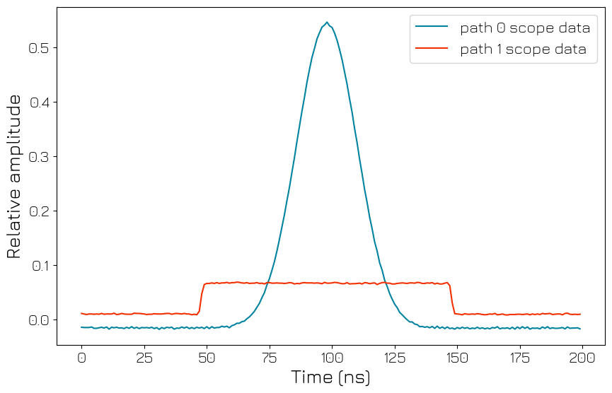
../../../_images/applications_setupguides_any_setupqbloxinstruments_61_0.png

Let’s make sense of this data.

We know that the output ranges of the QCM and QRM are $\simeq\pm 2.5V$ and $\simeq\pm 0.5V$, respectively. Since the input range of the QRM is $\simeq\pm 1V$, the recorded scope data values can be treated as the recorded signal voltage.

We generated an unmodulated square/block wave from QCM and QRM outputs with AWG amplitude $0.1$, meaning the signal output should be around $\simeq 0.25V$ and $\simeq 0.05V$ for the QCM and QRM respectively, which is exactly what we see.

We also see that the length of our pulse is $100$ ns, as expected.

Finally, we can appreciate the SYNQ at work, ensuring that both of the signals are perfectly synchronized.

Checking the Binned data#

Let’s also have a look at the binned data. As set before via Sequencer.integration_length_acq(), we know that the first 1000 scope values should be added and stored in the bin. Let’s verify this.

[26]:

bins = qrm_data["single"]["acquisition"]["bins"]

bins

[26]:

{'integration': {'path0': [0.8399217128753662], 'path1': [15.62859559059143]},
 'threshold': [1.0],
 'avg_cnt': [1]}

[27]:

print(
    "Sum of first 1000 path 0 scope values: ",
    sum(qrm_data["single"]["acquisition"]["scope"]["path0"]["data"][0:1000]),
)
print(
    "Sum of first 1000 path 1 scope values: ",
    sum(qrm_data["single"]["acquisition"]["scope"]["path1"]["data"][0:1000]),
)

Sum of first 1000 path 0 scope values:  0.84033203125
Sum of first 1000 path 1 scope values:  15.63623046875

We see that this is an exact match with the stored integrated bin values.

Including the QCM-RF#

Now, let’s add a QCM-RF to the mix.

We will generate a modulated Gaussian from the QCM-RF, using both the NCO and LO for upconversion.

Define waveforms#

[28]:

# Waveform parameters
waveform_length = 100  # nanoseconds

# Waveform dictionary (data will hold the samples and index will be used to select the waveforms in the instrument).
waveforms = {
    "gaussian": {
        "data": scipy.signal.windows.gaussian(waveform_length, std=0.12 * waveform_length).tolist(),
        "index": 0,
    },
    "block": {"data": [0.1 for i in range(0, waveform_length)], "index": 1},
    "zeros": {"data": [0.0 for i in range(0, waveform_length)], "index": 2},
}

Q1ASM program#

[29]:

qcm_rf_seq_prog = """

    ## Syncing with other sequencers
    wait_sync 4

    ## This is to enable the marker switch on the module, not to give an output from the marker channel.
    ## Since the microwave modules only have 2 output marker channels, the other 2 bits of the set_mrk
    ## instruction are reserved for the output switches of the modules. When these switches are turned off
    ## they act as 60dB attenuators
    set_mrk 3

    ## Playing a Gaussian envelope
    play 0,0,4

    stop

"""

For more details on how set_mrk works in the QCM-RF and QRM-RF, please see the Q1ASM instructions page.

Creating and uploading our sequence dictionary#

[30]:

# Add sequence to single dictionary
qcm_rf_sequence = {
    "waveforms": waveforms,
    "weights": {},
    "acquisitions": {},
    "program": qcm_rf_seq_prog,
}

qcm_rf.sequencer0.sequence(qcm_rf_sequence)

Configuring QCoDeS parameters via API#

SYNQ#

We add this sequencer to our SYNQ netowork as well.

[31]:

qcm_rf.sequencer0.sync_en(True)

Channel map#

[32]:

qcm_rf.disconnect_outputs()

qcm_rf.sequencer0.connect_out0("IQ")

Setting LO and NCO frequency#

We set the frequency of the output here via QCoDeS since we do not wish to dynamically modify it.

Note that the LO frequency can only be set via the API; that is, the LO is a static parameter in the QCM-RF and QRM-RF.

[33]:

# Enabling the LO for O1
qcm_rf.out0_lo_en(True)

# Setting the LO frequency for O1
qcm_rf.out0_lo_freq(3e9)

# Enabling the NCO and setting an NCO frequency for sequencer 0
qcm_rf.sequencer0.nco_freq(50e6)  # Equivalent to set_freq
qrm_rf.sequencer0.mod_en_awg(True)

Arming and starting all sequencers#

[34]:

# Arm and start all necessary sequencers

if qcms:
    qcm.arm_sequencer(0)

if qrms:
    qrm.arm_sequencer(0)
qcm_rf.arm_sequencer(0)

cluster.start_sequencer()

# Print status of all active sequencers.
if qcms:
    print(qcm.get_sequencer_status(0))
if qrms:
    print(qrm.get_sequencer_status(0))

if qcm_rfs:
    print(qcm_rf.get_sequencer_status(0))

Status: OKAY, State: STOPPED, Info Flags: NONE, Warning Flags: NONE, Error Flags: NONE, Log: []
Status: OKAY, State: STOPPED, Info Flags: ACQ_SCOPE_DONE_PATH_0, ACQ_SCOPE_DONE_PATH_1, ACQ_BINNING_DONE, Warning Flags: NONE, Error Flags: NONE, Log: []
Status: OKAY, State: STOPPED, Info Flags: NONE, Warning Flags: NONE, Error Flags: NONE, Log: []

Oscilloscope Output#

QCM_QRM_QCM_RF_scope_output

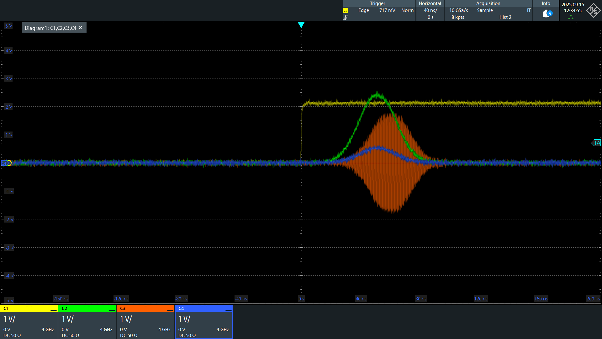
We see here that the output of the QCM-RF is slightly skewed relative to the baseband modules.

While SYNQ ensures that all sequencers added to the SYNQ network are synchronized, the RF modules have a slightly longer path length than the baseband modules, resulting in this skew. However, this skew can be eliminated by playing the RF signals earlier in the sequence.

Adding in the QRM-RF#

In this section, we will also include the QRM-RF.

We will output a square/block waveform that is upconverted by the NCO and LO, loop it back to the QRM-RF input, then downconvert and read out the signal.

We will study the acquired data after downconversion.

Define waveforms#

[35]:

# Waveform parameters
waveform_length = 100  # nanoseconds

# Waveform dictionary (data will hold the samples and index will be used to select the waveforms in the instrument).
waveforms = {
    "gaussian": {
        "data": scipy.signal.windows.gaussian(waveform_length, std=0.12 * waveform_length).tolist(),
        "index": 0,
    },
    "block": {"data": [0.1 for i in range(0, waveform_length)], "index": 1},
    "zeros": {"data": [0.0 for i in range(0, waveform_length)], "index": 2},
}

Q1ASM program#

[36]:

qrm_rf_seq_prog = """

    ## Syncing with all other sequencers
    wait_sync 4

    ## Setting output marker switches to on
    set_mrk 3

    ## Playing a block (index 1) on the I and Q channel
    play 1,1,4

    ## Acquiring the data
    acquire 0,0,4


    stop

"""

Creating and uploading the sequence#

Our acquisition dictionary can be identical to the one we used for the QRM, so we will directly create our sequence dictionary and upload.

[37]:

# Add sequence to single dictionary
qrm_rf_sequence = {
    "waveforms": waveforms,
    "weights": {},
    "acquisitions": qrm_acquisitions,
    "program": qrm_rf_seq_prog,
}

# Upload sequence.
qrm_rf.sequencer0.sequence(qrm_rf_sequence)

QCoDeS API settings#

SYNQ#

Adding the QRM-RF to the SYNQ network as well.

[38]:

# Configure the sequencers to synchronize.
qrm_rf.sequencer0.sync_en(True)

Channel map#

[39]:

# Map sequencers to specific outputs (but first disable all sequencer connections).
qrm_rf.disconnect_outputs()
qrm_rf.disconnect_inputs()

qrm_rf.sequencer0.connect_out0("IQ")
qrm_rf.sequencer0.connect_acq("in0")

Enabling scope acquisition#

Also, setting the integration length as before.

[40]:

# Configure scope mode
qrm_rf.scope_acq_sequencer_select(0)
qrm_rf.scope_acq_trigger_mode_path0("sequencer")
qrm_rf.scope_acq_trigger_mode_path1("sequencer")


# Configure integration
qrm_rf.sequencer0.integration_length_acq(1000)

Setting NCO and LO frequency#

[41]:

# Enabling modulation and demodulation by the NCO
qrm_rf.sequencer0.mod_en_awg(True)
qrm_rf.sequencer0.demod_en_acq(True)

# Setting the NCO frequency
qrm_rf.sequencer0.nco_freq(50e6)

# Enabling the LO and setting the LO frequency. If this is commented out, the value is set to the default value of 6Ghz
qrm_rf.out0_in0_lo_en(True)
qrm_rf.out0_in0_lo_freq(3e9)

Arming and starting the sequencers#

[42]:

# Arm and start all necessary sequencers.
if qcms:
    qcm.arm_sequencer(0)

if qrms:
    qrm.arm_sequencer(0)

if qcm_rfs:
    qcm_rf.arm_sequencer(0)

if qrm_rfs:
    qrm_rf.arm_sequencer(0)

cluster.start_sequencer()

# Print status of both sequencers.
if qcms:
    print(qcm.get_sequencer_status(0))

if qrms:
    print(qrm.get_sequencer_status(0))

if qcm_rfs:
    print(qcm_rf.get_sequencer_status(0))

print(qrm_rf.get_sequencer_status(0))

Status: OKAY, State: STOPPED, Info Flags: NONE, Warning Flags: NONE, Error Flags: NONE, Log: []
Status: OKAY, State: STOPPED, Info Flags: ACQ_SCOPE_DONE_PATH_0, ACQ_SCOPE_DONE_PATH_1, ACQ_BINNING_DONE, Warning Flags: NONE, Error Flags: NONE, Log: []
Status: OKAY, State: STOPPED, Info Flags: NONE, Warning Flags: NONE, Error Flags: NONE, Log: []
Status: OKAY, State: STOPPED, Info Flags: ACQ_SCOPE_DONE_PATH_0, ACQ_SCOPE_DONE_PATH_1, ACQ_BINNING_DONE, Warning Flags: NONE, Error Flags: NONE, Log: []

Lastly, adding the QTM#

For more details about QTM operation, please see the QTM scope mode tutorial and QTM binned mode tutorial.

In this section, we will see

How to output simple TTL pulses from the QTM
How to acquire the timetag for all rising edge events within a window using the QTM scope mode

QCoDeS API Settings#

We configure the various parameters needed for the output and input channels of the QTM.

[43]:

# Synchronize the two sequencers that will be used.
qtm.sequencer0.sync_en(True)
qtm.sequencer7.sync_en(True)

# Enable the output mode of the channel that we want to generate TTL pulses with.
qtm.io_channel0.mode("output")

# Enable the input mode of the channel we want to acquire with, and set the threshold level for event detection.
qtm.io_channel7.mode("input")
qtm.io_channel7.analog_threshold(1)  # This value is in volts


# Set the sequencer to trigger the scope mode.
qtm.io_channel7.scope_trigger_mode("sequencer")

# Set the scope mode to acquire all timetags within the acquisition window.
qtm.io_channel7.scope_mode("timetags-windowed")

Q1ASM program#

We must write 2 Q1ASM programs here: one for generating the TTL pulses, and 1 for acquiring them.

[44]:

qtm_program_pulse = """

    ## Syncing this sequencer with all the others
    wait_sync       4

    wait 100

    ## Setting the output to high for 100 ns
    set_digital 1,1,0  # level (1=high), mask (always 1), fine_delay in steps of 1/128 ns
    upd_param   100

    ## Setting the output back to low and waiting for 100 ns
    set_digital 0,1,0  # level (0=low), mask (always 1), fine_delay in steps of 1/128 ns
    upd_param 100

    ## Second pulse, also 100 ns long
    set_digital 1,1,0  # level (1=high), mask (always 1 for v1), fine_delay in steps of 1/128 ns
    upd_param   100

    ## Output back to low
    set_digital 0,1,0
    upd_param   4

    stop
"""

For more details about any of these Q1ASM instructions please see the Q1ASM instructions page.

[45]:

qtm_program_acq = """

    ## Synchronization
    wait_sync   4


    ## Opening the acquisition window for 1000 ns.
    acquire_timetags 0, 0, 1, 0, 4 # Data is stored at acq_index=0, bin_index=0.Argument 3 toggles the acquisition window. The total duration (4 + 996 of the next instruction) defines the window length.
    wait 996
    acquire_timetags 0, 0, 0, 0, 4

    stop
"""

Creating and uploading the sequence dictionaries#

[46]:

# Define acquisition dictionary.
qtm_acquisition_modes: dict[str, dict[str, int]] = {
    "timetag_single": {"num_bins": 1, "index": 0},
}
# Upload the pulse program to the sequencer.
qtm.sequencer0.sequence(
    {
        "waveforms": {},
        "weights": {},
        "acquisitions": {},
        "program": qtm_program_pulse,
    }
)
# Upload the acquisitions and program to the sequencer.
qtm.sequencer7.sequence(
    {
        "waveforms": {},
        "weights": {},
        "acquisitions": qtm_acquisition_modes,
        "program": qtm_program_acq,
    }
)

Arming and starting the sequencers#

[47]:

# Arm and starting all necessary sequencers.

qtm.sequencer0.arm_sequencer()
qtm.sequencer7.arm_sequencer()

if qcms:
    qcm.arm_sequencer(0)

if qrms:
    qrm.arm_sequencer(0)

if qcm_rfs:
    qcm_rf.arm_sequencer(0)

if qrm_rfs:
    qrm_rf.arm_sequencer(0)

cluster.start_sequencer()

# Print status of all active sequencers.
if qcms:
    print(qcm.get_sequencer_status(0))

if qrms:
    print(qrm.get_sequencer_status(0))

if qcm_rfs:
    print(qcm_rf.get_sequencer_status(0))

if qrm_rfs:
    print(qrm_rf.get_sequencer_status(0))

print(qtm.get_sequencer_status(0))
print(qtm.get_sequencer_status(7))

Status: OKAY, State: STOPPED, Info Flags: NONE, Warning Flags: NONE, Error Flags: NONE, Log: []
Status: OKAY, State: STOPPED, Info Flags: ACQ_SCOPE_DONE_PATH_0, ACQ_SCOPE_DONE_PATH_1, ACQ_BINNING_DONE, Warning Flags: NONE, Error Flags: NONE, Log: []
Status: OKAY, State: STOPPED, Info Flags: NONE, Warning Flags: NONE, Error Flags: NONE, Log: []
Status: OKAY, State: STOPPED, Info Flags: ACQ_SCOPE_DONE_PATH_0, ACQ_SCOPE_DONE_PATH_1, ACQ_BINNING_DONE, Warning Flags: NONE, Error Flags: NONE, Log: []
Status: OKAY, State: STOPPED, Info Flags: NONE, Warning Flags: NONE, Error Flags: NONE, Log: []
Status: ERROR, State: STOPPED, Info Flags: ACQ_BINNING_DONE, Warning Flags: NONE, Error Flags: DIO_TIME_DELTA_INVALID, Log: []

Fetching the acquired data#

Let’s check if the acquisition finished successfully.

[48]:

qtm.get_acquisition_status(7, 1)

[48]:

True

Let us fetch the scope data from the QTM and see what it looks like.

[49]:

scope_data = qtm.io_channel7.get_scope_data()
scope_data

[49]:

[['OPEN', 56996152860672], ['CLOSE', 56996154908672]]

We see that the returned data is simply a list of the timetag events recorded by the QTM. Here

'OPEN' and 'CLOSE' refer to the opening and closing of the acquisition window respectively. We will see below that the acquisition window closed exactly 1000 ns after opening.
'RISE' refers to recorded rising edge events that correspond to the start of the TTL pulses sent out by the QTM.
The returned timetag data is recorded in units of $\frac{1}{2048}$ nanoseconds. Note that the absolute value of the timetag has no meaning since we did not set an epoch.

[50]:

scope_data = np.zeros((3, 3)) if scope_data == 0 else scope_data
print(f"Number of acquired timetags in window: {len(scope_data)}")

# Convert the units of timetags to us.
timetags = np.array([(i[1] - scope_data[0][1]) / (2048) for i in scope_data])  # in nanoseconds


fig, ax = plt.subplots(1, 1)

for i in range(len(timetags)):
    if scope_data[i][0] == "OPEN":
        ax.plot(timetags[i], 1.0, marker="X", color="g", label="Window open")

    elif scope_data[i][0] == "CLOSE":
        ax.plot(timetags[i], 1.0, marker="X", color="r", label="Window close")

    elif scope_data[i][0] == "RISE":
        ax.plot(timetags[i], 1.0, marker="o", color="blue")

ax.set_xlabel(r"Time ($\mu$s)")
ax.set_ylabel("Photon detection")

plt.grid()
plt.legend()
plt.show()

Number of acquired timetags in window: 2

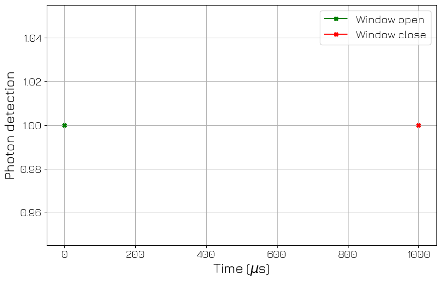
../../../_images/applications_setupguides_any_setupqbloxinstruments_119_1.png

Let’s check if the acquired timetags match the expected timetags.

[51]:

rich.print("All timetags in ns (relative to the first): ", timetags)
rich.print(
    "Difference between the arrival of the 2 TTL pulses = ", timetags[1] - timetags[0], " ns"
)

All timetags in ns (relative to the first):  [   0. 1000.]

Difference between the arrival of the 2 TTL pulses =  1000.0  ns

Hence, we can see that the recorded timetags are indeed correct. We see that the difference in the arrival of the two rising edges is 200 ns, and the acquisition window was closed 1000 ns after the start.

Stop everything#

[52]:

# Stop all sequencers.
cluster.stop_sequencer()

# Print status of all sequencers (should now say it is stopped).
if qcms:
    print(qcm.get_sequencer_status(0))

if qrms:
    print(qrm.get_sequencer_status(0))

if qcm_rfs:
    print(qcm_rf.get_sequencer_status(0))

if qrm_rfs:
    print(qrm_rf.get_sequencer_status(0))

if qtms:
    print(qtm.get_sequencer_status(0))
    print(qtm.get_sequencer_status(7))

# Uncomment below lines to print an overview of the instrument parameters.
# print("Snapshot:")
# qcm.print_readable_snapshot(update=True)
# qrm.print_readable_snapshot(update=True)
# qcm_rf.print_readable_snapshot(update=True)
# qrm_rf.print_readable_snapshot(update=True)
# qtm.print_readable_snapshot(update=True)

# Reset the cluster
cluster.reset()
print(cluster.get_system_status())

Status: OKAY, State: STOPPED, Info Flags: FORCED_STOP, Warning Flags: NONE, Error Flags: NONE, Log: []
Status: OKAY, State: STOPPED, Info Flags: FORCED_STOP, ACQ_SCOPE_DONE_PATH_0, ACQ_SCOPE_DONE_PATH_1, ACQ_BINNING_DONE, Warning Flags: NONE, Error Flags: NONE, Log: []
Status: OKAY, State: STOPPED, Info Flags: FORCED_STOP, Warning Flags: NONE, Error Flags: NONE, Log: []
Status: OKAY, State: STOPPED, Info Flags: FORCED_STOP, ACQ_SCOPE_DONE_PATH_0, ACQ_SCOPE_DONE_PATH_1, ACQ_BINNING_DONE, Warning Flags: NONE, Error Flags: NONE, Log: []
Status: OKAY, State: STOPPED, Info Flags: NONE, Warning Flags: NONE, Error Flags: NONE, Log: []
Status: ERROR, State: STOPPED, Info Flags: ACQ_BINNING_DONE, Warning Flags: NONE, Error Flags: DIO_TIME_DELTA_INVALID, Log: []
Status: ERROR, Flags: FEEDBACK_NETWORK_CALIBRATION_FAILED, Slot flags: SLOT2_FEEDBACK_NETWORK_CALIBRATION_FAILED, SLOT4_FEEDBACK_NETWORK_CALIBRATION_FAILED, SLOT6_FEEDBACK_NETWORK_CALIBRATION_FAILED, SLOT8_FEEDBACK_NETWORK_CALIBRATION_FAILED, SLOT10_FEEDBACK_NETWORK_CALIBRATION_FAILED, SLOT12_FEEDBACK_NETWORK_CALIBRATION_FAILED

Qblox Instruments Tutorial 0#

Standard Imports#

Connecting to the cluster#

Resetting the cluster#

Getting the relevant modules#

Selecting the modules#

Setup#

Only QCM#

Creating the waveforms dictionary#

Writing our Q1ASM sequence program#

Creating and Uploading the sequence dictionary#

Configuring QCoDeS (static and analog) parameters#

Adding the sequencer to the SYNQ network#

Channel Map#

Arming and starting the sequencer#

Oscilloscope Output#

QCM and QRM#

Define waveforms#

Q1ASM program#

Creating the acquisition dictionary#

Creating and uploading the sequence dictionary#

Configuring QCoDeS parameters via API#

Adding the sequencer to the SYNQ network#

Channel map#

Arming and starting the sequencers#

Oscilloscope Output#

Fetching the acquisition data from the QRM#

Plotting scope data#

Checking the Binned data#

Including the QCM-RF#

Define waveforms#

Q1ASM program#

Creating and uploading our sequence dictionary#

Configuring QCoDeS parameters via API#

SYNQ#

Channel map#

Setting LO and NCO frequency#

Arming and starting all sequencers#

Oscilloscope Output#

Adding in the QRM-RF#

Define waveforms#

Q1ASM program#

Creating and uploading the sequence#

QCoDeS API settings#

SYNQ#

Channel map#

Enabling scope acquisition#

Setting NCO and LO frequency#

Arming and starting the sequencers#

Lastly, adding the QTM#

QCoDeS API Settings#

Q1ASM program#

Creating and uploading the sequence dictionaries#

Arming and starting the sequencers#

Fetching the acquired data#

Stop everything#

Creating the `waveforms` dictionary#