See also
A Jupyter notebook version of this tutorial can be downloaded here.

Numerically Controlled Oscillator#
In this tutorial, we demonstrate how to exploit the dynamic capabilities of the FPGA to update frequency and phase in real time with a 1 ns time resolution.
Specifically, we will show how to use the numerically controlled oscillator (NCO) during an experiment to adjust the modulation frequency and apply phase updates. This is particularly useful for rapid spectroscopy measurements. Using the module’s sequencers, we will generate programmed waveforms on the outputs and simultaneously acquire the corresponding signals on the inputs. We will show this by using a QRC and directly connecting output \(\text{O}^{1}\) to input \(\text{I}^{1}\).
Whilst this tutorial is focused on the NCO, a similar procedure for spectroscopy over a wide frequency range with the LO can be found in the RF Control tutorial.
How the NCO works#
Modulation#
The NCO modulates the AWG output with a certain frequency, such that we only need to store the envelope of any waveform to create a wave with the correct frequency and phase. To enable IQ up- and down-conversion to RF frequencies, the device will generate a phase shifted signal on both signal paths.
If modulation is enabled, the value of the NCO (\(e^{i\omega t}\)) will be multiplied by the awg outputs (\(z(t) = \text{awg}_0 + i \cdot \text{awg}_1\)), and also by a factor of \(1 / \sqrt{2}\) to prevent clipping, and forwarded to path 0/1 as follows:
\begin{equation*} \text{path}_{0, \text{out}} = \frac{1}{\sqrt{2}}(\cos(\omega t)\text{awg}_0 - \sin(\omega t)\text{awg}_1) \end{equation*}
\begin{equation*} \text{path}_{1, \text{out}} = \frac{1}{\sqrt{2}}(\sin(\omega t)\text{awg}_0 + \cos(\omega t)\text{awg}_1) \end{equation*}
These two outputs can then be used within a QxM-RF module or by an external IQ mixer to generate RF pulses. Each path, 0/1, will have two components (real and imaginary) referred to as I and Q. However, the NCO can also be operated in real mode which will create a direct modulated output.
Demodulation#
When analyzing acquired signals, we are usually interested in their envelope rather than the full oscillating waveform—especially when integrating. To facilitate this, the NCO (Numerically Controlled Oscillator) can be used to demodulate the signal before integration.
If demodulation is enabled, the signal is multiplied by the NCO (effectively \(e^{-i\omega t}\) during demodulation), introducing a factor of \(\sqrt{2}\).
This results in a net amplitude factor of 1 for signals that are both modulated and demodulated—making the effect invisible to the user in standard use cases.
The relevant equations are:
Note
If only one path is used (for example, measuring a DC voltage with a QRM), this factor becomes visible. In such cases, the measured signal will appear larger by a factor of \(\sqrt{2}\) than it truly is.
Setup#
First, we are going to import the required packages and connect to the instrument.
[1]:
from __future__ import annotations

import json

import matplotlib.pyplot as plt
import numpy as np
from qcodes.instrument import find_or_create_instrument
from scipy.signal.windows import gaussian

from qblox_instruments import Cluster, ClusterType
Scan For Clusters#
We scan for the available devices connected via ethernet using the Plug & Play functionality of the Qblox Instruments package (see Plug & Play for more info).
!qblox-pnp list
[2]:
from typing import TYPE_CHECKING

if TYPE_CHECKING:
    from numpy.typing import NDArray
cluster_ip = "10.10.200.42"
cluster_name = "cluster0"
Connect to Cluster#
We now make a connection with the Cluster.
[3]:
cluster: Cluster = find_or_create_instrument(
    Cluster,
    recreate=True,
    name=cluster_name,
    identifier=cluster_ip,
    dummy_cfg=(
        {
            2: ClusterType.CLUSTER_QCM,
            4: ClusterType.CLUSTER_QRM,
            6: ClusterType.CLUSTER_QCM_RF,
            8: ClusterType.CLUSTER_QRM_RF,
            10: ClusterType.CLUSTER_QTM,
            12: ClusterType.CLUSTER_QRC,
            16: ClusterType.CLUSTER_QSM,
        }
        if cluster_ip is None
        else None
    ),
)

cluster.reset()
print(cluster.get_system_status())
Status: OKAY, Flags: NONE, Slot flags: NONE
Get connected modules#
[4]:
# QRC modules
modules = cluster.get_connected_modules(lambda mod: mod.is_qrc_type)
# This uses the module of the correct type with the lowest slot index
module = list(modules.values())[0]
Frequency sweeps#
One of the most common experiments is to test the frequency response of the system, e.g. to find the resonance frequencies of a qubit or a resonator. For the purpose of this tutorial, we will sweep the full frequency range of the NCO. To improve SNR we can use a long integration time and multiple averages.
[5]:
start_freq = -500e6
stop_freq = 500e6

n_averages = 10
MAXIMUM_SCOPE_ACQUISITION_LENGTH = 16384


def plot_amplitude_phase(x: NDArray, data: dict) -> None:
    I_data = (
        np.asarray(data["acquisition"]["bins"]["integration"]["path0"])
        / MAXIMUM_SCOPE_ACQUISITION_LENGTH
    )
    Q_data = (
        np.asarray(data["acquisition"]["bins"]["integration"]["path1"])
        / MAXIMUM_SCOPE_ACQUISITION_LENGTH
    )

    fig, ax = plt.subplots(1, 2)

    amplitude = np.abs(I_data + 1j * Q_data)
    phase = np.angle(I_data + 1j * Q_data)
    ax[0].plot(x / 1e6, amplitude)
    ax[1].plot(x / 1e6, phase)
    plt.xlabel("Frequency [MHz]")
    plt.ylabel("Integration [V]")
    plt.tight_layout()
    plt.show()


def plot_scope(trace: NDArray, t_min: int, t_max: int) -> None:
    if not np.any(trace):
        return
    x = np.arange(t_min, t_max)
    plt.plot(x, np.real(trace[t_min:t_max]))
    plt.plot(x, np.imag(trace[t_min:t_max]))
    plt.ylabel("Scope [V]")
    plt.xlabel("Time [ns]")
    plt.tight_layout()
    plt.show()
[6]:
module.disconnect_outputs()
module.disconnect_inputs()

# module.sequencer0.connect_sequencer("io0")
module.sequencer0.connect_out0("IQ")
module.sequencer0.connect_acq("in0")

module.sequencer0.nco_prop_delay_comp_en(True)

# The QRC has more input gain than other modules. To avoid overdriving the ADC, we set extra attenuation.
module.out0_att(20)
module.in0_att(20)

module.out0_in0_lo_freq(1e9)
module.sequencer0.nco_freq(50e6)
[7]:
# Enable hardware averaging for the scope
module.scope_acq_avg_mode_en_path0(True)
module.scope_acq_avg_mode_en_path1(True)

module.sequencer0.integration_length_acq(MAXIMUM_SCOPE_ACQUISITION_LENGTH)
Spectroscopy using Q1ASM#
Now we will run a spectroscopy experiment using Q1ASM to change the NCO frequency in real time. First, we set up the module for continuous wave output and binned acquisition with many bins. This is significantly faster than controlling it from the host PC. The maximum number of points that can be measured this way is on a sequencer is 3000000.
The sequencer program can fundamentally only support integer values. However, the NCO has a frequency resolution of 0.25 Hz and supports \(10^9\) phase values. Therefore, frequencies in the sequencer program must be given as integer multiple of \(1/4\) Hz, and phases as integer multiple of \(360/10^9\) degree.
[8]:
n_steps = 200

step_freq = (stop_freq - start_freq) / n_steps
print(f"{n_steps} steps with step size {step_freq / 1e6} MHz")

# Convert frequencies to multiples of 0.25 Hz
nco_int_start_freq = int(4 * start_freq)
nco_int_step_freq = int(4 * step_freq)
200 steps with step size 5.0 MHz
[9]:
acquisitions = {"acq": {"num_bins": n_steps, "index": 0}}

spectroscopy_program = f"""
    move {n_averages}, R2
    set_awg_offs    10000, 10000
    upd_param       200

avg_loop:
    move    {nco_int_start_freq}, R0          # frequency (may be negative)
    move    0, R1          # step counter

    reset_ph
    set_freq        R0
    upd_param       200

nco_set:
    set_freq        R0                           # Set the frequency
    add             R0, {nco_int_step_freq}, R0  # Update the frequency register
    upd_param       200                          # Wait for time of flight
    acquire         0, R1, {MAXIMUM_SCOPE_ACQUISITION_LENGTH}
    add             R1, 1, R1
    nop
    cmp             R1, {n_steps}
    jl              @nco_set                     # Loop over all frequencies

    sub             R2,1,R2
    jnz             @avg_loop

    stop                                  # Stop
"""

# Add sequence to single dictionary and write to JSON file.
sequence = {
    "waveforms": {},
    "weights": {},
    "acquisitions": acquisitions,
    "program": spectroscopy_program,
}
with open("sequence.json", "w", encoding="utf-8") as file:
    json.dump(sequence, file, indent=4)
Now we prepare the Module for measurement.
[10]:
module.sequencer0.sequence("sequence.json")

module.arm_sequencer(0)
module.start_sequencer()

print("Status:")
print(module.get_sequencer_status(0))

# Wait for the sequencer to stop with a timeout period of one minute.
module.get_acquisition_status(0, timeout=1)

data = module.get_acquisitions(0)["acq"]
Status:
Status: OKAY, State: RUNNING, Exit Code: 0, Info Flags: ACQ_SCOPE_DONE_PATH_0, ACQ_SCOPE_OVERWRITTEN_PATH_0, ACQ_SCOPE_DONE_PATH_1, ACQ_SCOPE_OVERWRITTEN_PATH_1, ACQ_BINNING_DONE, ACQ_SCOPE_DONE_PATH_2, ACQ_SCOPE_OVERWRITTEN_PATH_2, ACQ_SCOPE_DONE_PATH_3, Warning Flags: ACQ_SCOPE_OUT_OF_RANGE_PATH_0, ACQ_SCOPE_OUT_OF_RANGE_PATH_1, ACQ_INTEGRATOR_OUT_OF_RANGE_PATH_0, ACQ_INTEGRATOR_OUT_OF_RANGE_PATH_1, Error Flags: NONE, Log: []
[11]:
# For plotting, convert the NCO integer values back to frequencies
nco_sweep_range = (np.arange(n_steps) * nco_int_step_freq + nco_int_start_freq) / 4.0

plot_amplitude_phase(nco_sweep_range, data)

NCO input delay compensation#
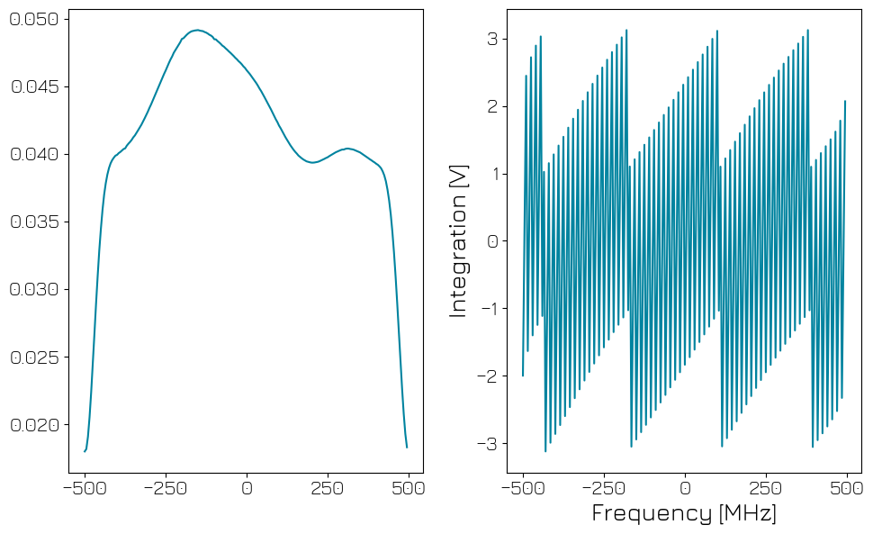
By default, the input and output of the QRM are multiplied with the same NCO value. As the output path has a time of flight between the NCO and playback, this means that there is a frequency-dependent relative phase between playback and demodulation. By enabling propagation delay compensation and matching to the time of flight, this phase can be removed. We will demonstrate this by running the same sequence as before, now with delay compensation enabled.
[12]:
module.sequencer0.nco_prop_delay_comp_en(True)

module.arm_sequencer(0)
module.start_sequencer()

print("Status:")
print(module.get_sequencer_status(0))

# Wait for the sequencer to stop with a timeout period of one minute.
module.get_acquisition_status(0, timeout=1)

data = module.get_acquisitions(0)["acq"]
Status:
Status: OKAY, State: RUNNING, Exit Code: 0, Info Flags: ACQ_SCOPE_DONE_PATH_0, ACQ_SCOPE_OVERWRITTEN_PATH_0, ACQ_SCOPE_DONE_PATH_1, ACQ_SCOPE_OVERWRITTEN_PATH_1, ACQ_BINNING_DONE, ACQ_SCOPE_DONE_PATH_2, ACQ_SCOPE_OVERWRITTEN_PATH_2, ACQ_SCOPE_DONE_PATH_3, Warning Flags: ACQ_SCOPE_OUT_OF_RANGE_PATH_0, ACQ_SCOPE_OUT_OF_RANGE_PATH_1, ACQ_INTEGRATOR_OUT_OF_RANGE_PATH_0, ACQ_INTEGRATOR_OUT_OF_RANGE_PATH_1, Error Flags: NONE, Log: []
[13]:
nco_sweep_range = (np.arange(n_steps) * nco_int_step_freq + nco_int_start_freq) / 4.0

plot_amplitude_phase(nco_sweep_range, data)
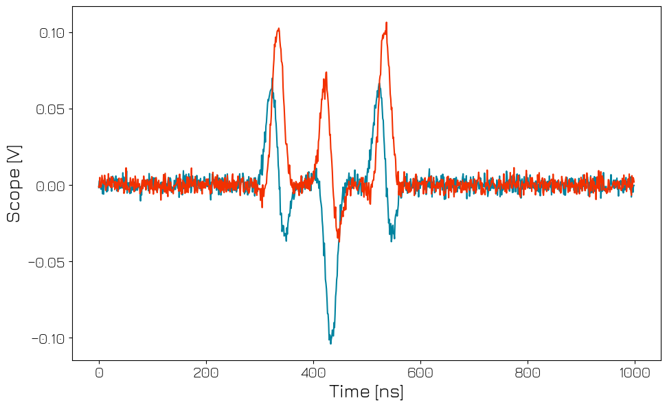
Phase updates#
In addition to fast frequency updates, the sequencer also supports real-time changes of the NCO phase. In particular for superconducting qubits, this can be used for a so-called virtual \(Z\) gate, see McKay et al. (2016). The virtual \(Z\) gate is a change of reference frame rather than a physical operation. Therefore, it is instantaneous and near perfect - the dominant error being that the NCO has a finite resolution of \(10^9\) different phases. Below, we will demonstrate how to to use a virtual Z to use the same pulse for both \(X\) and \(Y\) rotations.
As the sequencer internally only supports integer values, we must first convert the phase into an integer multiple of \(360/10^{9}\) degree:
[14]:
# Waveforms
waveform_len = 100
waveforms = {
    "gaussian": {
        "data": gaussian(waveform_len, std=0.133 * waveform_len).tolist(),
        "index": 0,
    },
}

# Acquisitions
acquisitions = {"scope": {"num_bins": 1, "index": 0}}

# Program
virtual_z = f"""
acquire         0,0,4
reset_ph
play            0,0,{waveform_len}      # X90
# This is equivalent to Y90, but uses the same waveform as X90
set_ph_delta    {int(90 * (1e9 / 360))}     # Z90
play            0,0,{waveform_len}      # X90
set_ph_delta    {int(270 * (1e9 / 360))}    # Z-90
play            0,0,{waveform_len}      # X90
stop
"""

# Write sequence to file.
with open("sequence.json", "w", encoding="utf-8") as file:
    json.dump(
        {
            "waveforms": waveforms,
            "weights": {},
            "acquisitions": acquisitions,
            "program": virtual_z,
        },
        file,
        indent=4,
    )
    file.close()
Now we can run the program and look at the scope acquisition.
[15]:
# Start the sequence
module.sequencer0.sequence("sequence.json")

module.arm_sequencer(0)
module.start_sequencer()

# Wait for the sequencer to stop with a timeout period of one minute
module.get_acquisition_status(0, timeout=1)

# Get acquisition data
module.store_scope_acquisition(0, "scope")
acq = module.get_acquisitions(0)

trace = np.asarray(acq["scope"]["acquisition"]["scope"]["path0"]["data"]) + 1j * np.asarray(
    acq["scope"]["acquisition"]["scope"]["path1"]["data"]
)

plot_scope(trace, 0, 1000)
Stop#
Finally, let’s stop the sequencers if they haven’t already and close the instrument connection. One can also display a detailed snapshot containing the instrument parameters before closing the connection by uncommenting the corresponding lines.
[16]:
# Stop all sequencers.
module.stop_sequencer()

# Print status of sequencers 0 and 1 (should now say it is stopped).
print(module.get_sequencer_status(0))
print(module.get_sequencer_status(1))
print()
Status: OKAY, State: STOPPED, Exit Code: 0, Info Flags: FORCED_STOP, ACQ_SCOPE_DONE_PATH_0, ACQ_SCOPE_DONE_PATH_1, ACQ_BINNING_DONE, ACQ_SCOPE_DONE_PATH_2, ACQ_SCOPE_DONE_PATH_3, Warning Flags: ACQ_SCOPE_OUT_OF_RANGE_PATH_0, ACQ_SCOPE_OUT_OF_RANGE_PATH_1, ACQ_INTEGRATOR_OUT_OF_RANGE_PATH_0, ACQ_INTEGRATOR_OUT_OF_RANGE_PATH_1, Error Flags: NONE, Log: []
Status: OKAY, State: STOPPED, Exit Code: 0, Info Flags: NONE, Warning Flags: NONE, Error Flags: NONE, Log: []