See also
A Jupyter notebook version of this tutorial can be downloaded here.

05 : Charge Stability Diagram#
Tutorial Objective#
The charge stability diagram provides a map of the stable electron configurations in a double quantum dot system as a function of gate voltages. By simultaneously sweeping two gate electrodes that tune the electrochemical potentials of the dots, and monitoring the response with a nearby charge sensor, one obtains a characteristic pattern of polygonal regions. Each region corresponds to a distinct charge occupation, while the boundaries mark transitions where electrons tunnel into or out of the dots. The geometry of these patterns reveals the interplay of Coulomb interactions, tunnel couplings, and gate lever arms, and serves as a key diagnostic for tuning and characterizing coupled quantum dot devices. For further information, see Hanson.2007.
Imports
[1]:
from __future__ import annotations

import rich  # noqa:F401

from qblox_scheduler import HardwareAgent, Schedule
from qblox_scheduler.operations import (
    Measure,
    SquarePulse,
)
from qblox_scheduler.operations.expressions import DType
from qblox_scheduler.operations.loop_domains import arange, linspace
/.venv/lib/python3.14/site-packages/quantify_core/utilities/general.py:13: QCoDeSDeprecationWarning: The `qcodes.utils.helpers` module is deprecated. Please consult the api documentation at https://microsoft.github.io/Qcodes/api/index.html for alternatives.
  from qcodes.utils.helpers import NumpyJSONEncoder
Hardware/Device Configuration Files#
We use JSON files in order to set the configurations for different parts of the whole system.
Hardware configuration
The hardware configuration file contains the cluster IP and the type of modules in that specific cluster (by cluster slot). Options such as the output attenuations, mixer corrections or LO frequencies can be fixed inside this file and the cluster will adapt to these settings when initialized. Hardware connectivities are also described here: Each module’s output is directly connected to the corresponding device port on the chip, allowing the software to address device elements directly and eliminating an extra layer of complexity for the user.
Device configuration
The device configuration file defines each quantum element and its associated properties. In this case, the basic spin elements are qubits, whilst the charge sensor element is a sensor and edges can be defined as barriers between the dots. As can be observed in this file, each element contains several key properties that can be pre-set in the file, or from within the Jupyter notebook (e.g. sensor.measure.pulse_amp(0.5)). Please have a quick look through these properties and change them as suited to your device, if needed. Some of the typically important properties are: acq_delay, integration_time, and clock_freqs. You may also adjust the default pulse amplitudes and pulse durations for a given element here, or may define additional elements as needed.
Using the information specified in these files, we set the hardware and device configurations which determines the connectivity of our system.
[2]:
hw_config_path = "dependencies/configs/tuning_spin_coupled_pair_hardware_config.json"
device_path = "dependencies/configs/spin_with_psb_device_config_2q.yaml"
Experimental Setup#
To run the tutorial, you will need a quantum device consists of a double quantum dot array (q0 and q1), with a charge sensor (cs0) connected to reflectometry readout. The DC voltages of the quantum device also need to be properly tuned. For example, reservoir gates need to be ramped up for the accumulation devices. The charge sensor can be a quantum dot, quantum point contact (QPC), or single electron transistor (SET).
The HardwareAgent() is the main object for Qblox experiments. It provides an interface to define the quantum device, set up hardware connectivity, run experiments, and receive results.
[3]:
hw_agent = HardwareAgent(hw_config_path, device_path)
hw_agent.connect_clusters()

# Device name string should be defined as specified in the hardware configuration file
sensor_0 = hw_agent.quantum_device.get_element("cs0")
qubit_0 = hw_agent.quantum_device.get_element("q0")
qubit_1 = hw_agent.quantum_device.get_element("q1")
/.venv/lib/python3.14/site-packages/qblox_scheduler/qblox/hardware_agent.py:485: UserWarning: cluster0: Trying to instantiate cluster with ip 'None'.Creating a dummy cluster.
  warnings.warn(
As can be observed from the defined quantum devices and the hardware connectivies of these elements, the relevant modules and connections for this tutorial are:
QCM (Module 2):
\(\text{O}^{1}\): Gate connection line for qubit 0 (
q0).\(\text{O}^{2}\): Gate connection line for qubit 1 (
q1).
QRM (Module 4):
\(\text{O}^{1}\) and \(\text{I}^{1}\): Charge sensor (
cs0) resonator probe and readout connection.
Charge Stability Diagram - Schedule & Measurement#
We define a measurement sequence for mapping out a charge stability diagram.
This schedule performs a 2D sweep over two plunger gate voltages applied to target_element_1 and target_element_2. For each amplitude pair, gate voltage pulses are applied simultaneously, and a charge sensor measurement is used to detect transitions in the charge configuration of the system.
We define all variables for the experiment schedule in one location for ease of access and modification.
[4]:
repetitions = 2
pulse_duration = 100e-8
target_element_1 = qubit_0
target_element_2 = qubit_1
sensor = sensor_0
[5]:
charge_stability_schedule = Schedule("2-parameter sweep")

ref_op = None
with (
    charge_stability_schedule.loop(arange(0, repetitions, 1, DType.NUMBER)),
    charge_stability_schedule.loop(
        linspace(
            start=0.0,
            stop=0.5,
            num=3,
            dtype=DType.AMPLITUDE,
        )
    ) as amp1,
    charge_stability_schedule.loop(
        linspace(start=0.0, stop=0.75, num=2, dtype=DType.AMPLITUDE)
    ) as amp2,
):
    ref_op = charge_stability_schedule.add(
        SquarePulse(
            amp=amp1,
            duration=pulse_duration,
            port=target_element_1.ports.gate,
        ),
        ref_op=ref_op,
    )
    charge_stability_schedule.add(
        SquarePulse(
            amp=amp2,
            duration=pulse_duration,
            port=target_element_2.ports.gate,
        ),
        ref_op=ref_op,
        ref_pt="start",
    )
    charge_stability_schedule.add(
        Measure(
            sensor.name,
            gate_pulse_amp=0.5,
            coords={"port1_amplitude": amp1, "port2_amplitude": amp2},
            acq_channel="Sensor_Response",
        ),
        ref_op=ref_op,
        ref_pt="start",
    )
Now, we will run the schedule. See the documentation on the QRM Module and Readout Sequencers for information on how the signal is processed upon acquisition.
Note that this schedule can be adapted to perform a concurrent sweep of any two output ports by changing the sweep objects (with the exception of ChargeSensor elements).
[6]:
charge_stability_ds = hw_agent.run(charge_stability_schedule)
charge_stability_ds
[6]:
<xarray.Dataset> Size: 288B
Dimensions:                          (acq_index_Sensor_Response: 6)
Coordinates:
  * acq_index_Sensor_Response        (acq_index_Sensor_Response) int64 48B 0 ...
    port2_amplitude                  (acq_index_Sensor_Response) float64 48B ...
    loop_repetition_Sensor_Response  (acq_index_Sensor_Response) float64 48B ...
    port1_amplitude                  (acq_index_Sensor_Response) float64 48B ...
Data variables:
    Sensor_Response                  (acq_index_Sensor_Response) complex128 96B ...
Attributes: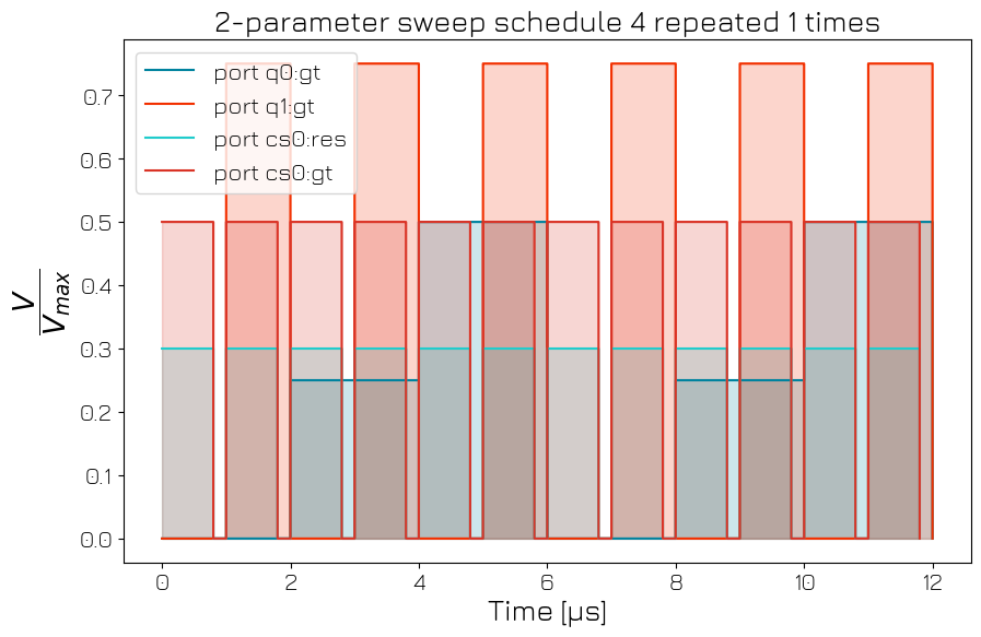
tuid: 20260204-002655-817-8c98cdYou may plot the pulse diagram of a schedule for verification.
[7]:
hw_agent.compile(charge_stability_schedule).plot_pulse_diagram()
[7]:
(<Figure size 1000x621 with 1 Axes>,
 <Axes: title={'center': '2-parameter sweep schedule 4 repeated 1 times'}, xlabel='Time [μs]', ylabel='$\\dfrac{V}{V_{max}}$'>)
The quantum device settings can be saved after every experiment for allowing later reference into experiment settings.
[8]:
hw_agent.quantum_device.to_json_file("./dependencies/configs", add_timestamp=True)
[8]:
'./dependencies/configs/spin_with_psb_device_config_2026-02-04_00-26-56_UTC.json'