See also
A Jupyter notebook version of this tutorial can be downloaded here.
01 : Time of Flight Measurement#
Tutorial Objective#
In this tutorial, we aim to measure the time of flight (in other words, the propagation delay between the output and the input of the control system). Knowing the time of flight is essential for synchronizing control & readout pulses with the quantum system’s response, ensuring correct timing and phase alignment in experiments. Thus, the analysis of the data obtained from this application example will be useful to calibrate the acquisition delay for subsequent experiments, improving the quality of the digitized signal.
Imports#
[1]:
import rich  # noqa:F401
from dependencies.analysis_utils import TimeOfFlightAnalysis
from dependencies.simulated_data import get_tof_data

from qblox_scheduler import HardwareAgent, Schedule
from qblox_scheduler.backends.qblox import constants
from qblox_scheduler.math import closest_number_ceil
from qblox_scheduler.operations import Measure, SetClockFrequency
from qblox_scheduler.operations.expressions import DType
from qblox_scheduler.operations.loop_domains import arange
/.venv/lib/python3.14/site-packages/quantify_core/utilities/general.py:13: QCoDeSDeprecationWarning: The `qcodes.utils.helpers` module is deprecated. Please consult the api documentation at https://microsoft.github.io/Qcodes/api/index.html for alternatives.
  from qcodes.utils.helpers import NumpyJSONEncoder
Hardware/Device Configuration Files#
We use JSON files in order to set the configurations for different parts of the whole system.
Hardware configuration
The hardware configuration file contains the cluster IP and the type of modules in that specific cluster (by cluster slot). Options such as the output attenuations, mixer corrections or LO frequencies can be fixed inside this file and the cluster will adapt to these settings when initialized. Hardware connectivities are also described here: Each module’s output is directly connected to the corresponding device port on the chip, allowing the software to address device elements directly and eliminating an extra layer of complexity for the user.
Device configuration
The device configuration file defines each quantum element and its associated properties. In this case, the basic spin elements are qubits, whilst the charge sensor element is a sensor and edges can be defined as barriers between the dots. As can be observed in this file, each element contains several key properties that can be pre-set in the file, or from within the Jupyter notebook (e.g. sensor.measure.pulse_amp(0.5)). Please have a quick look through these properties and change them as suited to your device, if needed. Some of the typically important properties are: acq_delay, integration_time, and clock_freqs. You may also adjust the default pulse amplitudes and pulse durations for a given element here, or may define additional elements as needed.
Using the information specified in these files, we set the hardware and device configurations which determines the connectivity of our system.
[2]:
hw_config_path = "dependencies/configs/tuning_spin_coupled_pair_hardware_config.json"
device_path = "dependencies/configs/spin_with_psb_device_config_2q.yaml"
Experimental Setup#
To run the tutorial, you will need a quantum device consists of a double quantum dot array (q0 and q1), with a charge sensor (cs0) connected to reflectometry readout. The DC voltages of the quantum device also need to be properly tuned. For example, reservoir gates need to be ramped up for the accumulation devices. The charge sensor can be a quantum dot, quantum point contact (QPC), or single electron transistor (SET).
The HardwareAgent() is the main object for Qblox experiments. It provides an interface to define the quantum device, set up hardware connectivity, run experiments, and receive results.
[3]:
hw_agent = HardwareAgent(hw_config_path, device_path)
hw_agent.connect_clusters()

# Device name string should be defined as specified in the hardware configuration file
sensor_0 = hw_agent.quantum_device.get_element("cs0")
cluster = hw_agent.get_clusters()["cluster0"]
hw_opts = hw_agent.hardware_configuration.hardware_options
/.venv/lib/python3.14/site-packages/qblox_scheduler/qblox/hardware_agent.py:485: UserWarning: cluster0: Trying to instantiate cluster with ip 'None'.Creating a dummy cluster.
  warnings.warn(
As can be observed from the defined quantum devices and the hardware connectivies of these elements, the relevant modules and connections for this tutorial are:
QRM (Module 4):
\(\text{O}^{1}\) and \(\text{I}^{1}\): Charge sensor (
cs0) resonator probe and readout connection.
Time of Flight - Schedule & Measurement#
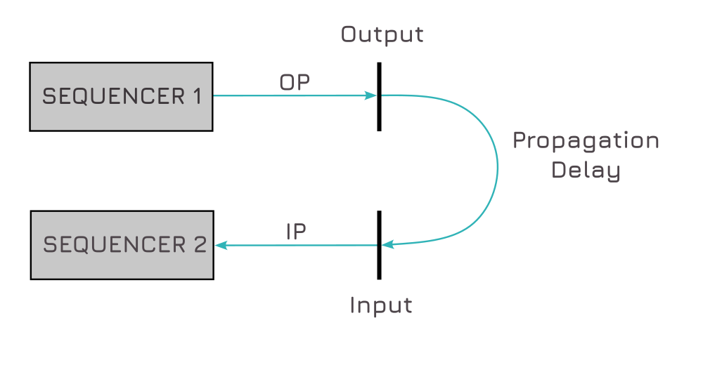
Prior to the start of quantum experiments, it is crucial to calibrate the delay between sending a measurement pulse and the beginning of the acquisition on the instrument. This delay should be equal to the time it takes for the readout signal to travel through the fridge and is determined by the length of the cables, as well as other delay inducing components. In order to perform the experiment, a square pulse is played over the output of the readout line, and a trace acquisition is done. The time at which the pulse is detected on the acquisition path is determined as the acquisition delay. This also allows us to set the NCO propagation delay, which corrects for the phase accumulated during the time of flight.
We define all variables for the experiment schedule in one location for ease of access and modification.
[4]:
sensor = sensor_0
repetitions = 500
[5]:
# Define a schedule and set the repetition rate
tof_schedule = Schedule("Trace measurement schedule")
# Set the clock frequency of the sensor readout port
with tof_schedule.loop(arange(0, repetitions, 1, DType.NUMBER)):
    tof_schedule.add(
        SetClockFrequency(
            clock=sensor.name + ".ro", clock_freq_new=sensor.clock_freqs.readout - 100e6
        )  # We detune clock 100MHz from the expected resonance frequency, at which the signal will be partially absorbed.
    )
    # Acquire a trace of the signal acquired at the input port
    tof_schedule.add(Measure(sensor.name, acq_protocol="Trace", acq_channel="chan_0"))
Now, we will run the schedule. See the documentation on the QRM Module and Readout Sequencers for information on how the signal is processed upon acquisition.
[6]:
hw_opts.output_att.update({f"{sensor.name}.ro": 0})  # set attenuation to zero to have max signal
tof_data = hw_agent.run(tof_schedule)
tof_data
[6]:
<xarray.Dataset> Size: 16kB
Dimensions:             (acq_index_chan_0: 1, trace_index_chan_0: 650)
Coordinates:
  * acq_index_chan_0    (acq_index_chan_0) int64 8B 0
  * trace_index_chan_0  (trace_index_chan_0) int64 5kB 0 1 2 3 ... 647 648 649
Data variables:
    chan_0              (acq_index_chan_0, trace_index_chan_0) complex128 10kB ...
Attributes:
tuid: 20260204-002732-248-510c06Analysis#
[7]:
# Add simulated data in case a dummy cluster is being used. This is done in order to successfully showcase the expected results of an analysis in all cases.
if cluster.is_dummy:
    tof_data.chan_0.data = get_tof_data(sensor.measure.integration_time)[0].reshape(
        1, len(tof_data.chan_0.data[0])
    )

tof_analysis = TimeOfFlightAnalysis(
    dataset=tof_data,
)
tof_analysis.run().display_figs_mpl()
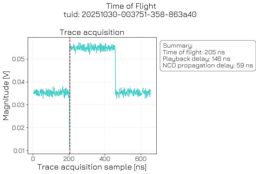
The analysis yields the time of flight in the system: The time difference between the beginning of the acquisition and the actual incidence of the acquired signal on the acquisition port. This result should be considered when the acquisition delay parameter is configured for subsequent experiments in order to avoid integrating over a portion of the noise floor signal before the actual signal from the experiment is acquired. Thus, we set the acquisition delay of the sensor according to the information we obtain from data analysis.
[8]:
fit_results = tof_analysis.quantities_of_interest
nco_prop_delay = fit_results["nco_prop_delay"]
measured_tof = fit_results["tof"]

sensor.measure.acq_delay = (
    closest_number_ceil(
        measured_tof * constants.SAMPLING_RATE, constants.MIN_TIME_BETWEEN_OPERATIONS
    )
    / constants.SAMPLING_RATE
)
The quantum device settings can be saved after every experiment for allowing later reference into experiment settings.
[9]:
hw_agent.quantum_device.to_json_file("./dependencies/configs", add_timestamp=True)
[9]:
'./dependencies/configs/spin_with_psb_device_config_2026-02-04_00-27-33_UTC.json'