See also
A Jupyter notebook version of this tutorial can be downloaded here.

06a : PSB Readout#
Tutorial Objective#
The objective of this tutorial is to demonstrate how to perform the Pauli Spin Blockade (PSB) readout on a double quantum dot system. For further information on this readout method, see Barthel.2009.
Imports
[1]:
from __future__ import annotations

import rich  # noqa:F401
from dependencies.psb import OperatingPoints, PsbEdge

from qblox_scheduler import (
    HardwareAgent,
    Schedule,
)
from qblox_scheduler.operations import (
    Measure,
    PulseCompensation,
    RampPulse,
    SquarePulse,
)
/.venv/lib/python3.14/site-packages/quantify_core/utilities/general.py:13: QCoDeSDeprecationWarning: The `qcodes.utils.helpers` module is deprecated. Please consult the api documentation at https://microsoft.github.io/Qcodes/api/index.html for alternatives.
  from qcodes.utils.helpers import NumpyJSONEncoder
Hardware/Device Configuration Files#
We use JSON files in order to set the configurations for different parts of the whole system.
Hardware configuration
The hardware configuration file contains the cluster IP and the type of modules in that specific cluster (by cluster slot). Options such as the output attenuations, mixer corrections or LO frequencies can be fixed inside this file and the cluster will adapt to these settings when initialized. Hardware connectivities are also described here: Each module’s output is directly connected to the corresponding device port on the chip, allowing the software to address device elements directly and eliminating an extra layer of complexity for the user.
Device configuration
The device configuration file defines each quantum element and its associated properties. In this case, the basic spin elements are qubits, whilst the charge sensor element is a sensor and edges can be defined as barriers between the dots. As can be observed in this file, each element contains several key properties that can be pre-set in the file, or from within the Jupyter notebook (e.g. sensor.measure.pulse_amp(0.5)). Please have a quick look through these properties and change them as suited to your device, if needed. Some of the typically important properties are: acq_delay, integration_time, and clock_freqs. You may also adjust the default pulse amplitudes and pulse durations for a given element here, or may define additional elements as needed.
Using the information specified in these files, we set the hardware and device configurations which determines the connectivity of our system.
[2]:
hw_config_path = "dependencies/configs/tuning_spin_coupled_pair_hardware_config.json"
device_path = "dependencies/configs/spin_with_psb_device_config_2q.yaml"
Experimental Setup#
To run the tutorial, you will need a quantum device consists of a double quantum dot array (q0 and q1), with a charge sensor (cs0) connected to reflectometry readout. The DC voltages of the quantum device also need to be properly tuned. For example, reservoir gates need to be ramped up for the accumulation devices. The charge sensor can be a quantum dot, quantum point contact (QPC), or single electron transistor (SET).
The HardwareAgent() is the main object for Qblox experiments. It provides an interface to define the quantum device, set up hardware connectivity, run experiments, and receive results.
[3]:
hw_agent = HardwareAgent(hw_config_path, device_path)
hw_agent.connect_clusters()

# Device name string should be defined as specified in the hardware configuration file
sensor_0 = hw_agent.quantum_device.get_element("cs0")
qubit_0 = hw_agent.quantum_device.get_element("q0")
qubit_1 = hw_agent.quantum_device.get_element("q1")
hw_opts = hw_agent.hardware_configuration.hardware_options
cluster = hw_agent._clusters["cluster0"].cluster
/.venv/lib/python3.14/site-packages/qblox_scheduler/qblox/hardware_agent.py:485: UserWarning: cluster0: Trying to instantiate cluster with ip 'None'.Creating a dummy cluster.
  warnings.warn(
As can be observed from the defined quantum devices and the hardware connectivies of these elements, the relevant modules and connections for this tutorial are:
QCM (Module 2):
\(\text{O}^{1}\): Gate connection line for qubit 0 (
q0).\(\text{O}^{2}\): Gate connection line for qubit 1 (
q1).
QRM (Module 4):
\(\text{O}^{1}\) and \(\text{I}^{1}\): Charge sensor (
cs0) resonator probe and readout connection.\(\text{O}^{2}\) : Charge sensor (
cs0) plunger gate connection.
PSB Readout#
In order to apply PSB Readout in a concise and readable manner, we implement a custom defined ‘’’Edge’’’ that is configured for this purpose. For details on how to configure such a custom device element or edge, see the Make Your Own Device Elements tutorial.
[4]:
q0_q1 = PsbEdge(qubit_0, qubit_1)

q0_q1.control.parent_voltage = 0.1
q0_q1.control.child_voltage = -0.2
q0_q1.control.barrier_voltage = 0.3

q0_q1.readout.parent_voltage = 0.0
q0_q1.readout.child_voltage = 0.0
q0_q1.readout.barrier_voltage = 0.0

hw_agent.quantum_device.add_edge(q0_q1)
We further introduce two helper functions to be able to move along or hold at certain points of the charge stability diagram:
``ramps`` Creates a schedule that smoothly ramps the voltages from one operating point to another using
RampPulse. The duration of the ramp is determined by theRampingTimessubmodule of thePSBEdge.``hold`` Creates a schedule that holds the system at a given operating point for a fixed duration using
SquarePulse. This is useful when you want to keep the system stable at a specific bias point (e.g., during readout).
Both functions loop over the parameters defined in the operating points (e.g. control and readout points and both for qubits and barrier gates), fetch the corresponding hardware ports, and then generate the appropriate pulses. This further helps with readability and streamlining of the generated schedules, which are expected to include PSB Readout quite frequently.
[5]:
def ramps(op_start: OperatingPoints, op_end: OperatingPoints) -> Schedule:
    """Generate a schedule to ramp gate voltages between two PSB operating points."""
    parent = op_start.parent
    port_dict = parent.port_dict
    ramp_time = parent.ramps.to_dict()[f"{op_start.name}_to_{op_end.name}"]

    ops = op_start.to_dict()
    ope = op_end.to_dict()

    sched = Schedule("")
    ref_op = None
    for key in op_start.parameters:
        amplitude = ope[key] - ops[key]
        offset = ops[key]
        ref_op = sched.add(
            RampPulse(amp=amplitude, offset=offset, duration=ramp_time, port=port_dict[key]),
            ref_pt="start",
            ref_op=ref_op,
        )
    return sched


def hold(op_point: OperatingPoints, duration: float) -> Schedule:
    """Generate a schedule to hold gate voltages at a given PSB operating point."""
    parent = op_point.parent
    port_dict = parent.port_dict

    sched = Schedule("")
    ref_op = None
    for key in op_point.parameters:
        ref_op = sched.add(
            SquarePulse(amp=op_point.to_dict()[key], duration=duration, port=port_dict[key]),
            ref_pt="start",
            ref_op=ref_op,
        )
    return sched
PSB Readout - Schedule & Measurement#
Using the PSBEdge and the helper functions defined above, we generate a compact schedule for implementing a PSB Readout experiment.
We define all variables for the experiment schedule in one location for ease of access and modification.
[6]:
sensor = sensor_0
[7]:
schedule = Schedule(
    ""
)  # Define an schedule to be given as a body to the pulse compensated schedule. This schedule will include the bulk of the experiment.
psb_readout_schedule = Schedule("Pulse Compensated Schedule")

schedule.add(ramps(q0_q1.readout, q0_q1.control))
schedule.add(hold(q0_q1.control, 200e-9))
schedule.add(ramps(q0_q1.control, q0_q1.readout))
ref_pulse_measure = schedule.add(hold(q0_q1.readout, sensor.measure.pulse_duration))
schedule.add(Measure(sensor.name), ref_op=ref_pulse_measure, ref_pt="start")
psb_readout_schedule.add(
    PulseCompensation(
        schedule,
        max_compensation_amp={
            "q0:gt": 0.110,
            "q1:gt": 0.120,
            "q0_q1:gt": 0.09,
            "cs0:gt": 0.09,
        },
        time_grid=4e-9,
        sampling_rate=1e9,
    )
)
[7]:
{'name': '0c3eb092-de2b-4132-8039-a5e9274758d5', 'operation_id': '7244206528751575340', 'timing_constraints': [TimingConstraint(ref_schedulable=None, ref_pt=None, ref_pt_new=None, rel_time=0)], 'label': '0c3eb092-de2b-4132-8039-a5e9274758d5'}
Now, we will run the schedule. See the documentation on the QRM Module and Readout Sequencers for information on how the signal is processed upon acquisition.
[8]:
psb_readout_ds = hw_agent.run(psb_readout_schedule)
psb_readout_ds
[8]:
<xarray.Dataset> Size: 24B
Dimensions:      (acq_index_0: 1)
Coordinates:
  * acq_index_0  (acq_index_0) int64 8B 0
Data variables:
    0            (acq_index_0) complex128 16B (nan+nanj)
Attributes: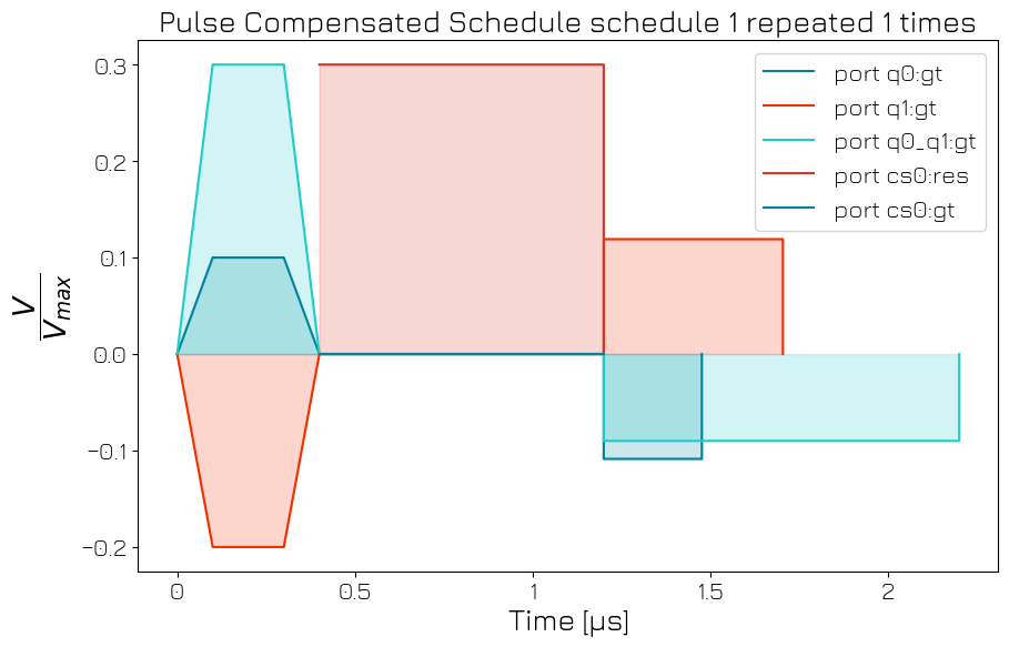
tuid: 20260204-002641-401-f63d7fYou may plot the pulse diagram of a schedule for verification.
[9]:
hw_agent.compile(psb_readout_schedule).plot_pulse_diagram()
[9]:
(<Figure size 1000x621 with 1 Axes>,
 <Axes: title={'center': 'Pulse Compensated Schedule schedule 1 repeated 1 times'}, xlabel='Time [μs]', ylabel='$\\dfrac{V}{V_{max}}$'>)
The quantum device settings can be saved after every experiment for allowing later reference into experiment settings.
[10]:
hw_agent.quantum_device.to_json_file("./dependencies/configs", add_timestamp=True)
[10]:
'./dependencies/configs/spin_with_psb_device_config_2026-02-04_00-26-42_UTC.json'