See also
A Jupyter notebook version of this tutorial can be downloaded here.

04a : Coulomb Peaks#
Objectives#
In this tutorial, we measure charge sensor’s Coulomb peaks. The sharp conductance gradient of Coulomb peaks makes them ideal sensors for the electrostatic state of nearby quantum dots.
Imports
[1]:
from __future__ import annotations

import numpy as np
import rich  # noqa:F401

from qblox_scheduler import HardwareAgent, Schedule
from qblox_scheduler.operations import Measure, PulseCompensation, SquarePulse
/.venv/lib/python3.14/site-packages/quantify_core/utilities/general.py:13: QCoDeSDeprecationWarning: The `qcodes.utils.helpers` module is deprecated. Please consult the api documentation at https://microsoft.github.io/Qcodes/api/index.html for alternatives.
  from qcodes.utils.helpers import NumpyJSONEncoder
Hardware/Device Configuration Files#
We use JSON files in order to set the configurations for different parts of the whole system.
Hardware configuration
The hardware configuration file contains the cluster IP and the type of modules in that specific cluster (by cluster slot). Options such as the output attenuations, mixer corrections or LO frequencies can be fixed inside this file and the cluster will adapt to these settings when initialized. Hardware connectivities are also described here: Each module’s output is directly connected to the corresponding device port on the chip, allowing the software to address device elements directly and eliminating an extra layer of complexity for the user.
Device configuration
The device configuration file defines each quantum element and its associated properties. In this case, the basic spin elements are qubits, whilst the charge sensor element is a sensor and edges can be defined as barriers between the dots. As can be observed in this file, each element contains several key properties that can be pre-set in the file, or from within the Jupyter notebook (e.g. sensor.measure.pulse_amp(0.5)). Please have a quick look through these properties and change them as suited to your device, if needed. Some of the typically important properties are: acq_delay, integration_time, and clock_freqs. You may also adjust the default pulse amplitudes and pulse durations for a given element here, or may define additional elements as needed.
Using the information specified in these files, we set the hardware and device configurations which determines the connectivity of our system.
[2]:
hw_config_path = "dependencies/configs/tuning_spin_coupled_pair_hardware_config.json"
device_path = "dependencies/configs/spin_with_psb_device_config_2q.yaml"
Experimental Setup#
To run the tutorial, you will need a quantum device consists of a double quantum dot array (q0 and q1), with a charge sensor (cs0) connected to reflectometry readout. The DC voltages of the quantum device also need to be properly tuned. For example, reservoir gates need to be ramped up for the accumulation devices. The charge sensor can be a quantum dot, quantum point contact (QPC), or single electron transistor (SET).
The HardwareAgent() is the main object for Qblox experiments. It provides an interface to define the quantum device, set up hardware connectivity, run experiments, and receive results.
[3]:
hw_agent = HardwareAgent(hw_config_path, device_path)
hw_agent.connect_clusters()

# Device name string should be defined as specified in the hardware configuration file
sensor_0 = hw_agent.quantum_device.get_element("cs0")
qubit_0 = hw_agent.quantum_device.get_element("q0")
qubit_1 = hw_agent.quantum_device.get_element("q1")
/.venv/lib/python3.14/site-packages/qblox_scheduler/qblox/hardware_agent.py:485: UserWarning: cluster0: Trying to instantiate cluster with ip 'None'.Creating a dummy cluster.
  warnings.warn(
Modules are connected to the quantum device via:
QCM (Module 2):
\(\text{O}^{1}\): plunger gate of qubit 0 (
q0).\(\text{O}^{2}\): plunger gate of qubit 1 (
q1).
QRM (Module 4):
\(\text{O}^{1}\) and \(\text{I}^{1}\): resonator of the charge sensor (
cs0).
Schedule & Measurement#
We will now build the schedule for a 1D gate voltage sweep. The goal is to find Coulomb peaks by applying a pulse with a varying amplitude to target element and recording the cs0’s response.
The schedule’s behavior changes depending on what you define as the target_element: To find a dot’s peaks (Cross-Capacitance): If the target_element is a quantum dot (e.g., q0), the schedule does two things for each amplitude: Pulse: Applies a square pulse to the dot’s gate. Measure: After a short delay, it sends a separate pulse to the sensor to measure its response.
To calibrate the sensor (Self-Sweep): If the target_element is the sensor itself, the logic is simpler. For each amplitude, the schedule applies a single measurement pulse to the sensor, using the swept amplitude as its gate_pulse_amp. This “self-sweep” is the method we use to find the sensor’s own Coulomb peaks and identify its most sensitive working point.
We define all variables for the experiment schedule in one location for ease of access and modification.
[4]:
repetitions = 101
sensor = sensor_0
target_element = sensor_0
pulse_duration = 800e-9
amplitudes = np.linspace(0.02, 0.9, 7)
[5]:
coulomb_peaks_schedule = Schedule("pulse_compensation", repetitions=repetitions)

# Make sure the element that is assigned to obtain data is a charge sensor
if not sensor.__class__.__name__ == "ChargeSensor":
    raise ValueError("The measure object is not a charge sensor object.")

# Sweep over pulse amplitude of the gate port of the target element in the given amplitude range, and obtain the charge sensor response for every amplitude value.
for amp in amplitudes:
    inner_schedule = Schedule("schedule", repetitions=1)
    if target_element == sensor:
        inner_schedule.add(Measure(sensor.name, gate_pulse_amp=amp, pulse_duration=pulse_duration))
    else:
        inner_schedule.add(
            SquarePulse(amp=amp, duration=pulse_duration, port=target_element.ports.gate)
        )
        inner_schedule.add(
            Measure(
                sensor.name,
                gate_pulse_amp=sensor.measure.pulse_amp,
            ),
            rel_time=250e-9,
        )  # rel_time defines the time between this Measure() operation and the previous SquarePulse() operation

    # Add pulse compensation
    coulomb_peaks_schedule.add(
        PulseCompensation(
            inner_schedule,
            max_compensation_amp={"q0:gt": 0.110, "q1:gt": 0.120, "cs0:gt": 0.15},
            time_grid=4e-9,
            sampling_rate=1e9,
        )
    )
Now, we will run the schedule. See the documentation on the QRM Module and Readout Sequencers for information on how the signal is processed upon acquisition.
Before running this schedule, please make sure that the measurement pulse amplitude, duration, acquisition delay and integration time parameters are adjusted to your needs in the device configuration file. These will be defined via the sensor device (in this case, named “cs0”) since the measurement is performed at the device level.
Note that this schedule can be adapted to perform a sweep of the gate connection of any quantum device element via changing the target element.
[6]:
coulomb_peaks_ds = hw_agent.run(coulomb_peaks_schedule)
coulomb_peaks_ds
[6]:
<xarray.Dataset> Size: 168B
Dimensions:      (acq_index_0: 7)
Coordinates:
  * acq_index_0  (acq_index_0) int64 56B 0 1 2 3 4 5 6
Data variables:
    0            (acq_index_0) complex128 112B (nan+nanj) ... (nan+nanj)
Attributes: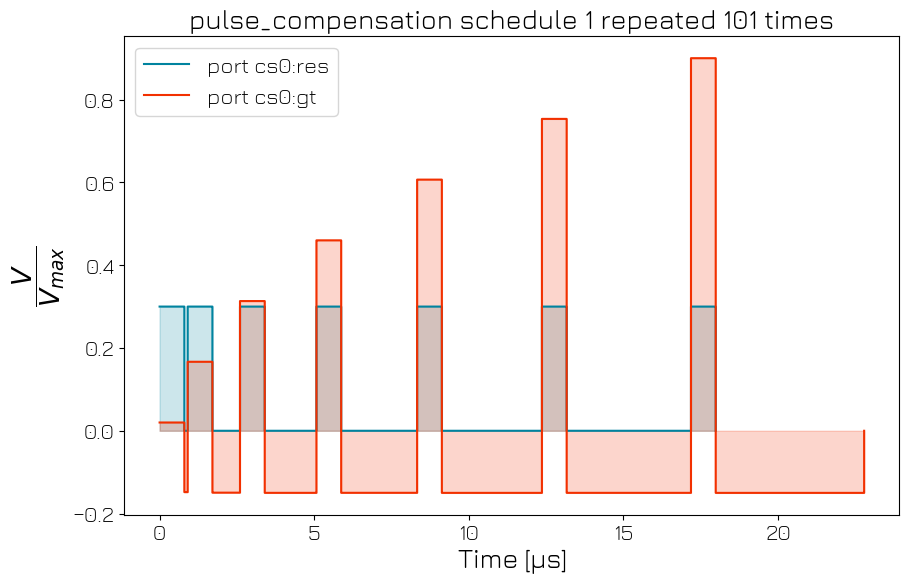
tuid: 20260204-002741-132-4126cbYou may plot the pulse diagram of a schedule for verification.
[7]:
hw_agent.compile(coulomb_peaks_schedule).plot_pulse_diagram()
[7]:
(<Figure size 1000x621 with 1 Axes>,
 <Axes: title={'center': 'pulse_compensation schedule 1 repeated 101 times'}, xlabel='Time [μs]', ylabel='$\\dfrac{V}{V_{max}}$'>)
The quantum device settings can be saved after every experiment for allowing later reference into experiment settings.
[8]:
hw_agent.quantum_device.to_json_file("./dependencies/configs", add_timestamp=True)
[8]:
'./dependencies/configs/spin_with_psb_device_config_2026-02-04_00-27-41_UTC.json'