03: Correcting for signal distortions due to Bias Tee#

Introducing BIAS Tee#

The Bias-T (Bias Tee) is a diplexer consisting of an inductor and a capacitor. As shown below, the capacitor port (also known as the RF port) allows the passage of high-frequency components while attenuating the low-frequency elements of the signal. In contrast, the inductor port (also known as the DC port) allows a DC signal to pass through. The output port combines the RF and DC inputs.

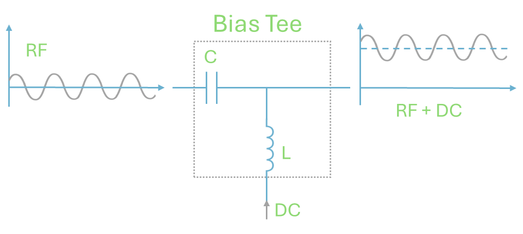
A Bias-T is essential for spin qubit systems, especially when combining a small RF signal with a large DC offset. This configuration allows for significant attenuation of the RF line to minimize noise, while the DC component is filtered through a series of filters and the Bias-T itself.

However, the Bias-T, being a filter, inevitably introduces signal distortion that can compromise the waveform sent to the qubit. In this demo we showcase how to mitigate these undesirable effects, which manifest as an exponential decay visible on both long and short timescales (relative to the Bias-T’s time constant). We will present two optimized solutions, one for each scenario.

Additionally, we will validate these improvements by applying the corrections to a real Bias-T and comparing the output on the oscilloscope with our simulated results.

Imports

[1]:

from __future__ import annotations

import matplotlib.pyplot as plt
import numpy as np
import rich  # noqa:F401
from dependencies._030_net_zero.bias_tee_utils import (
    bias_tee_correction,
    bias_tee_distort,
    get_axis,
    plot_waveform_and_rectangle,
)

from qblox_scheduler import HardwareAgent, Schedule
from qblox_scheduler.operations import (
    NumericalPulse,
    PulseCompensation,
    RampPulse,
    SquarePulse,
)

Hardware/Device Configuration Files#

We use JSON files in order to set the configurations for different parts of the whole system.

Using the information specified in these files, we set the hardware and device configurations which determines the connectivity of our system.

[2]:

hw_config_path = "dependencies/configs/tuning_spin_coupled_pair_hardware_config.json"
device_path = "dependencies/configs/spin_with_psb_device_config_2q.yaml"

Experimental Setup#

To run the tutorial, you will need a quantum device consists of a double quantum dot array (q0 and q1), with a charge sensor (cs0) connected to reflectometry readout. The DC voltages of the quantum device also need to be properly tuned. For example, reservoir gates need to be ramped up for the accumulation devices. The charge sensor can be a quantum dot, quantum point contact (QPC), or single electron transistor (SET).

The HardwareAgent() is the main object for Qblox experiments. It provides an interface to define the quantum device, set up hardware connectivity, run experiments, and receive results.

[3]:

hw_agent = HardwareAgent(hw_config_path, device_path)
hw_agent.connect_clusters()

qubit_0 = hw_agent.quantum_device.get_element("q0")

/builds/0/.venv/lib/python3.10/site-packages/qblox_scheduler/qblox/hardware_agent.py:460: UserWarning: cluster0: Trying to instantiate cluster with ip 'None'.Creating a dummy cluster.
  warnings.warn(

Schedule definition#

The schedule_function consists of two schedules:

The uncompensated_sched schedule plays the instrument’s output directly without any correction.
The compensated_sched schedule employs the PulseCompensation operation with the net-zero protocol to mitigate the Bias-T’s long-term decay effects. This operation calculates the required compensation pulse parameters, including amplitude and duration, and inserts the compensation pulse after the main schedule body has executed.

[4]:

def schedule_function(
    port: str,
    amp_points: np.ndarray,
    square_dur: float,
    ramp_dur: float,
    second_square_dur: float,
    reps: int = 1,
) -> tuple[Schedule, Schedule]:
    """
    Generate uncompensated and compensated pulse schedules for a given port.

    This function creates two schedules:
    - An uncompensated schedule that directly applies a sequence of
      square and ramp pulses at different amplitude set points.
    - A compensated schedule that wraps the same sequence in a
      net-zero compensation protocol to reduce distortions.

    Args:
        port: Hardware port on which to play the pulses.
        amp_points: Array of amplitude set points for the ramp pulse.
        square_dur: Duration of the initial zero-amplitude square pulse (seconds).
        ramp_dur: Duration of the ramp pulse (seconds).
        second_square_dur: Duration of the second square pulse with current amplitude (seconds).
        reps: Number of times to repeat the full schedule. Defaults to 1.

    Returns:
        A tuple containing:
            - uncompensated_sched: The raw schedule without compensation.
            - compensated_sched: The schedule with pulse compensation applied.

    """
    uncompensated_sched = Schedule("uncompensated", repetitions=reps)
    compensated_sched = Schedule("compensated", repetitions=reps)

    # Loop through each amplitude set point
    for amp in amp_points:
        # Create a pulse sequence schedule
        pulse_sequence = Schedule("pulse_sequence")

        # Add a square pulse with zero amplitude
        pulse_sequence.add(SquarePulse(amp=0, duration=square_dur, port=port))

        # Add a ramp pulse with the current amplitude
        pulse_sequence.add(RampPulse(amp=amp, offset=0, duration=ramp_dur, port=port))

        # Add a second square pulse with the current amplitude
        pulse_sequence.add(SquarePulse(amp=amp, duration=second_square_dur, port=port))

        # Add the pulse sequence to the uncompensated schedule
        uncompensated_sched.add(pulse_sequence)

        # Add the pulse sequence with net-zero protocol to the compensated schedule
        compensated_sched.add(
            PulseCompensation(
                body=pulse_sequence,
                max_compensation_amp={port: 0.8},
                time_grid=4e-9,
                sampling_rate=1e9,
            )
        )

    return uncompensated_sched, compensated_sched

Set parameters for schedule_function

[5]:

decay = 17000  # Time constant for the Bias-T distortion in ns.
amp_set_points = np.linspace(0.02, 0.9, 10)  # Define an array of amplitude set points
square_duration = 300e-9  # Duration of the first square pulse in ns.
ramp_duration = 400e-9  # Duration of the ramp pulse in ns.
second_square_duration = 100e-9  # Duration of the second square pulse in ns.
repetitions = int(1e6)  # repetitions is 1e6 so that we can see it on the scope
port = qubit_0.ports.gate  # Port to use for the pulse sequence

Run the uncompensated schedule

[6]:

uncompensated_sched, _ = schedule_function(
    port,
    amp_set_points,
    square_duration,
    ramp_duration,
    second_square_duration,
    repetitions,
)

[7]:

# To verify this Bias-T behavior, we use a real device with a 17 µs decay (matching the simulation parameters).
#
# We connect the **QCM** output to the Bias-T's RF port and then connect the combined port to an oscilloscope.
# Then we run the uncompensated complied schedule `compiled_schedule_uncomp`.
uncompensated_ds = hw_agent.run(uncompensated_sched)

Plot the waveform

[8]:

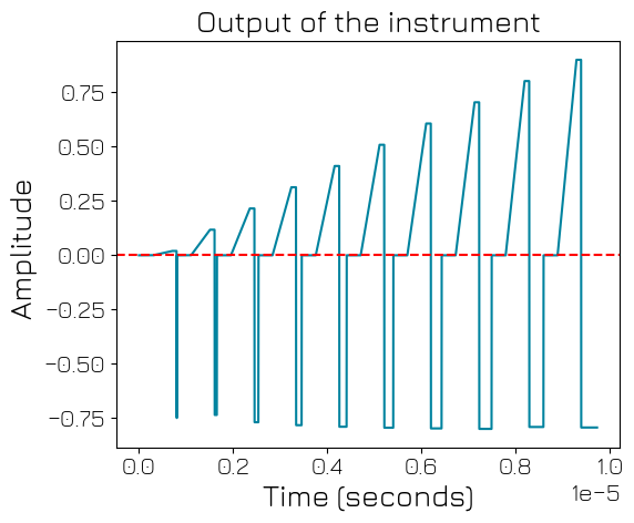
x, y = get_axis(hw_agent.compile(uncompensated_sched))
plot_waveform_and_rectangle(x, y, decay, second_square_duration, amp_set_points)

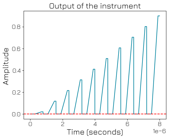
../../../_images/applications_spin_Spin_030_net_zero_17_0.png

../../../_images/applications_spin_Spin_030_net_zero_17_1.png

The second plot reveals a clear decay, both in the long-term mean value (indicated by the red dashed line) and on a shorter timescale within the highlighted region.

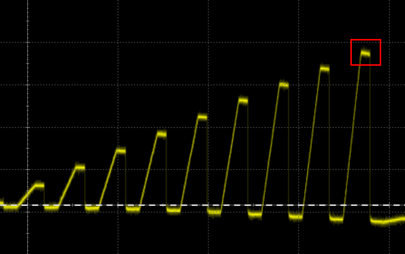
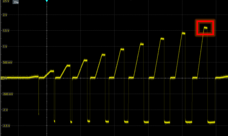
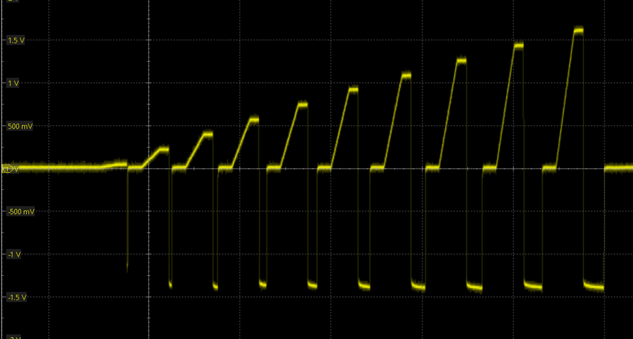
Scope output#

The output from the oscilloscope is shown below. Note that the effects of the Bias-T on both short and long pulses are clearly visible, closely matching our results from the simulation.

[9]:

hw_agent.instrument_coordinator.stop()

Compensating for long-term decay: `PulseCompensation`#

To see the effect of PulseCompensation operation, we compile and run the compensated_sched part of the schedule_function.

[10]:

_, compensated_sched = schedule_function(
    port,
    amp_set_points,
    square_duration,
    ramp_duration,
    second_square_duration,
    repetitions,
)

To confirm, we run the complied schedule compiled_schedule_net_zero with the real Bias-T, and observe the output at the scope. compensated_ds = hw_agent.run(compensated_sched)

[11]:

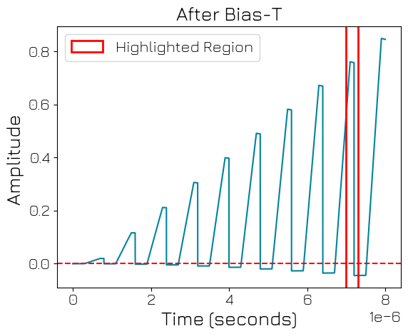
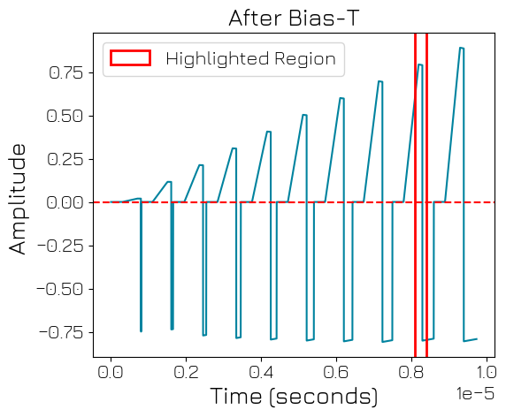
x, y = get_axis(hw_agent.compile(compensated_sched))
# Plot the waveform
new_y = plot_waveform_and_rectangle(x, y, decay, second_square_duration, amp_set_points)

../../../_images/applications_spin_Spin_030_net_zero_24_0.png

../../../_images/applications_spin_Spin_030_net_zero_24_1.png

Scope output#

The output figure above shows that the Net-zero protocol effectively compensates for the DC decay caused by the Bias-T, leaving only the short pulse distortion to be corrected (as seen in the highlighted region).

Mitigating short-term decay#

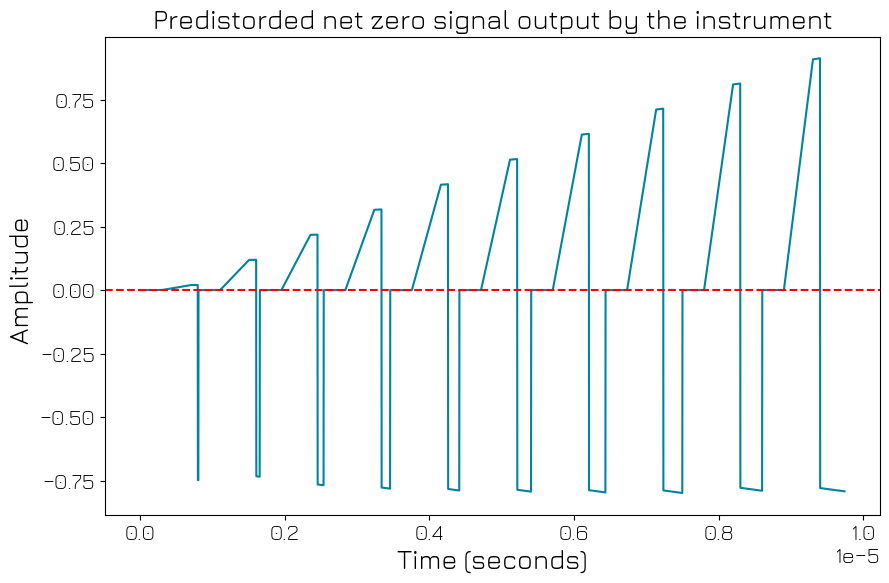
To perfectly account for the Bias-T, we use the function bias_tee_correction. It pre-distorts the signal to compensate for short-term decay. Hence, the resulting in the following waveform (shown in the plot).

[12]:

pre_distorded_signal = bias_tee_correction(y, decay)
plt.figure()
plt.title("Predistorded net zero signal output by the instrument")
plt.plot(x, pre_distorded_signal)
plt.axhline(0, c="red", linestyle="--")
plt.xlabel("Time (seconds)")
plt.ylabel("Amplitude ")

[12]:

Text(0, 0.5, 'Amplitude ')

../../../_images/applications_spin_Spin_030_net_zero_27_1.png

Finally, we send the pre-distorted waveform through a Bias-T, that is simulated using bias_tee_distort function. The resulted signal output is free from any Bias-T defects.

[13]:

final_compensated_signal = bias_tee_distort(pre_distorded_signal, decay)
plt.figure()
plt.title("Final output signal by the instrument after Bias-T")
plt.plot(x, final_compensated_signal, label="Final output after correction for Bias-T")
plt.axhline(0, c="red", linestyle="--")
plt.xlabel("Time (seconds)")
plt.ylabel("Amplitude ")

[13]:

Text(0, 0.5, 'Amplitude ')

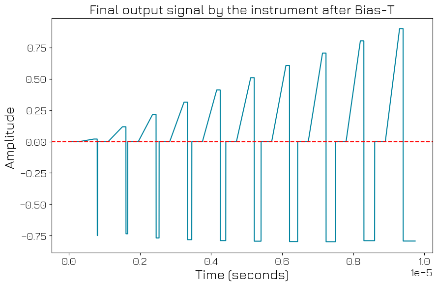
../../../_images/applications_spin_Spin_030_net_zero_29_1.png

Using this filter alone, one can also correct long-term decay. But this may clip the outputs, which is not recommended. Combining the Net-zero protocol with the Bias-T filter enables you to deliver the exact signal required for the QPU, without clipping the output.

To verify the pre-distortion with the real Bias-T, we initialize another schedule, final_compensated_sched. Here, we add the pre_distorded_signal using NumericalPulse. This allows us to play any arbitrary waveform.

[14]:

# Initialize the final schedule with a single repetition
final_compensated_sched = Schedule("final", repetitions=int(1e6))
t_x = (x * 1e9 // 4).astype(int) * 4  # sampling the time at 4 ns resolution

# Add a NumericalPulse to the schedule with the pre-distorted signal
final_compensated_sched.add(
    NumericalPulse(
        samples=pre_distorded_signal,  # The pre-distorted signal waveform
        t_samples=t_x * 1e-9,  # Time samples in seconds
        port=qubit_0.ports.gate,  # Port where the pulse is applied
    )
)

[14]:

{'name': 'bce9132b-8772-4365-834d-735c58cb5f82', 'operation_id': '3719511217020089337', 'timing_constraints': [TimingConstraint(ref_schedulable=None, ref_pt=None, ref_pt_new=None, rel_time=0)], 'label': 'bce9132b-8772-4365-834d-735c58cb5f82'}

[15]:

hw_agent.run(final_compensated_sched)

/builds/0/.venv/lib/python3.10/site-packages/scipy/interpolate/_interpolate.py:479: RuntimeWarning: invalid value encountered in divide
  slope = (y_hi - y_lo) / (x_hi - x_lo)[:, None]

[15]:

<xarray.Dataset> Size: 0B
Dimensions:  ()
Data variables:
    *empty*
Attributes:
    tuid:     20251030-003740-070-f8de9f

Scope output#

As shown in the output above, the final waveform is free from distortion in both the short and long pulse regimes.

If you want to try it with different Bias-T, make sure you change the time-constant variable decay accordingly in the above script.

[16]:

hw_agent.instrument_coordinator.stop()

03: Correcting for signal distortions due to Bias Tee#

Introducing BIAS Tee#

Hardware/Device Configuration Files#

Experimental Setup#

Schedule definition#

Scope output#

Compensating for long-term decay: PulseCompensation#

Scope output#

Mitigating short-term decay#

Scope output#

Compensating for long-term decay: `PulseCompensation`#