See also
A Jupyter notebook version of this tutorial can be downloaded here.

02: Resonator Spectroscopy#
Tutorial Objective#
If the readout procedure of the spin system is performed using RF reflectometry, impedance matching between the quantum dot device and the readout port is typically achieved via an LCR circuit.
The objective of this tutorial is to identify the resonance frequency of such a LCR circuit at which the effective impedance of the quantum-dot device is best matched to the 50 \(\Omega\) readout port (the characteristic impedance of standard coaxial cables and output ports of most experimental instruments). Around this resonance, small changes in the electrostatic potential of the sensor or quantum dots shift the effective impedance of the LCR circuit. These impedance shifts lead to measurable changes in the reflected RF signal, providing a sensitive readout mechanism.
Imports
[1]:
from __future__ import annotations

import numpy as np
import rich  # noqa:F401
from dependencies.analysis_utils import ResonatorSpectroscopyAnalysis
from dependencies.simulated_data import get_resonator_spec_data

from qblox_scheduler import HardwareAgent, Schedule
from qblox_scheduler.operations import (
    IdlePulse,
    Measure,
    SetClockFrequency,
    SSBIntegrationComplex,
    VoltageOffset,
)
from qblox_scheduler.operations.expressions import DType
from qblox_scheduler.operations.loop_domains import arange, linspace
from qblox_scheduler.resources import ClockResource
/.venv/lib/python3.14/site-packages/quantify_core/utilities/general.py:13: QCoDeSDeprecationWarning: The `qcodes.utils.helpers` module is deprecated. Please consult the api documentation at https://microsoft.github.io/Qcodes/api/index.html for alternatives.
  from qcodes.utils.helpers import NumpyJSONEncoder
Hardware/Device Configuration Files#
We use JSON files in order to set the configurations for different parts of the whole system.
Hardware configuration
The hardware configuration file contains the cluster IP and the type of modules in that specific cluster (by cluster slot). Options such as the output attenuations, mixer corrections or LO frequencies can be fixed inside this file and the cluster will adapt to these settings when initialized. Hardware connectivities are also described here: Each module’s output is directly connected to the corresponding device port on the chip, allowing the software to address device elements directly and eliminating an extra layer of complexity for the user.
Device configuration
The device configuration file defines each quantum element and its associated properties. In this case, the basic spin elements are qubits, whilst the charge sensor element is a sensor and edges can be defined as barriers between the dots. As can be observed in this file, each element contains several key properties that can be pre-set in the file, or from within the Jupyter notebook (e.g. sensor.measure.pulse_amp(0.5)). Please have a quick look through these properties and change them as suited to your device, if needed. Some of the typically important properties are: acq_delay, integration_time, and clock_freqs. You may also adjust the default pulse amplitudes and pulse durations for a given element here, or may define additional elements as needed.
Using the information specified in these files, we set the hardware and device configurations which determines the connectivity of our system.
[2]:
hw_config_path = "dependencies/configs/tuning_spin_coupled_pair_hardware_config.json"
device_path = "dependencies/configs/spin_with_psb_device_config_2q.yaml"
Experimental Setup#
To run the tutorial, you will need a quantum device consists of a double quantum dot array (q0 and q1), with a charge sensor (cs0) connected to reflectometry readout. The DC voltages of the quantum device also need to be properly tuned. For example, reservoir gates need to be ramped up for the accumulation devices. The charge sensor can be a quantum dot, quantum point contact (QPC), or single electron transistor (SET).
The HardwareAgent() is the main object for Qblox experiments. It provides an interface to define the quantum device, set up hardware connectivity, run experiments, and receive results.
[3]:
hw_agent = HardwareAgent(hw_config_path, device_path)
hw_agent.connect_clusters()

# Device name string should be defined as specified in the hardware configuration file
sensor_0 = hw_agent.quantum_device.get_element("cs0")
hw_opts = hw_agent.hardware_configuration.hardware_options
cluster = hw_agent.get_clusters()["cluster0"]
/.venv/lib/python3.14/site-packages/qblox_scheduler/qblox/hardware_agent.py:485: UserWarning: cluster0: Trying to instantiate cluster with ip 'None'.Creating a dummy cluster.
  warnings.warn(
As can be observed from the defined quantum devices and the hardware connectivies of these elements, the relevant modules and connections for this tutorial are:
QRM (Module 4):
\(\text{O}^{1}\) and \(\text{I}^{1}\): Charge sensor (
cs0) resonator probe and readout connection.
Pulsed Spectrocopy - Schedule & Measurement#
We define all variables for the experiment schedule in one location for ease of access and modification.
[4]:
repetitions = 301
center_frequency = 200 * 1e6
width = 75e6
frequencies = np.linspace(center_frequency - width / 2, center_frequency + width / 2, 300)
sensor = sensor_0
Schedule definition#
[5]:
res_spec_schedule = Schedule("Resonator Spectroscopy Schedule", repetitions=repetitions)

# Define a loop operation to sweep the frequency of the readout port signal.
with (
    res_spec_schedule.loop(arange(0, repetitions, 1, DType.NUMBER)),
    res_spec_schedule.loop(
        linspace(
            start=center_frequency - width / 2,
            stop=center_frequency + width / 2,
            num=300,
            dtype=DType.FREQUENCY,
        )
    ) as freq,
):
    res_spec_schedule.add(
        Measure(
            sensor.name,
            freq=freq,
            coords={"frequency": freq},
            acq_channel="chan_0",
        )
    )
    res_spec_schedule.add(IdlePulse(8e-9))
Now, we will run the schedule. See the documentation on the QRM Module and Readout Sequencers for information on how the signal is processed upon acquisition.
[6]:
res_spec_data = hw_agent.run(res_spec_schedule)
res_spec_data
[6]:
<xarray.Dataset> Size: 12kB
Dimensions:                 (acq_index_chan_0: 300)
Coordinates:
  * acq_index_chan_0        (acq_index_chan_0) int64 2kB 0 1 2 3 ... 297 298 299
    frequency               (acq_index_chan_0) float64 2kB 1.625e+08 ... 2.37...
    loop_repetition_chan_0  (acq_index_chan_0) float64 2kB 0.0 1.0 ... 299.0
Data variables:
    chan_0                  (acq_index_chan_0) complex128 5kB (nan+nanj) ... ...
Attributes:
tuid: 20260204-002750-105-7a2030Continuous Wave Spectrocopy - Schedule & Measurement#
In order to implement a continuous wave (CW) resonator spectroscopy schedule, we return to the pulse level expression instead of the gate level (e.g. the example above with a simple Measure()) gate. Pulse-level expression is applicable here since we will be sweeping the frequency over a continuous tone, which cannot be expressed as a gate operation.
We define all variables for the experiment schedule in one location for ease of access and modification.
[7]:
repetitions = 301
center_frequency = 220 * 1e6
width = 75e6
frequencies = np.linspace(center_frequency - width / 2, center_frequency + width / 2, 300)
sensor = sensor_0
clock = sensor.name + ".ro"
port = sensor.ports.readout
[8]:
cw_res_spec_schedule = Schedule(
    "Continuous Wave Resonator Spectroscopy Schedule", repetitions=repetitions
)

# Define a clock resource to adjust the clock frequency of the sensor readout port as needed
cw_res_spec_schedule.add_resource(ClockResource(name=sensor.name + ".ro", freq=center_frequency))
# Set a voltage offset to mimic a continuous wave spectroscopy experiment
cw_res_spec_schedule.add(VoltageOffset(offset_path_I=0.1, offset_path_Q=0, port=port, clock=clock))
cw_res_spec_schedule.add(IdlePulse(duration=4e-9))

# Define a loop operation to sweep the frequency of the readout port signal.
with (
    cw_res_spec_schedule.loop(arange(0, repetitions, 1, DType.NUMBER)),
    cw_res_spec_schedule.loop(
        linspace(
            start=center_frequency - width / 2,
            stop=center_frequency + width / 2,
            num=300,
            dtype=DType.FREQUENCY,
        )
    ) as freq,
):
    cw_res_spec_schedule.add(SetClockFrequency(clock=clock, clock_freq_new=freq))

    cw_res_spec_schedule.add(
        SSBIntegrationComplex(
            duration=sensor.measure.integration_time,
            port=port,
            clock=clock,
            coords={"frequency": freq},
            acq_channel="chan_0",
        )
    )

cw_res_spec_schedule.add(VoltageOffset(offset_path_I=0, offset_path_Q=0, port=port, clock=clock))
cw_res_spec_schedule.add(IdlePulse(duration=4e-9))
[8]:
{'name': '7dad08a9-09c8-4c86-a1ae-64be0175f52e', 'operation_id': '-3991725939193774227', 'timing_constraints': [TimingConstraint(ref_schedulable=None, ref_pt=None, ref_pt_new=None, rel_time=0)], 'label': '7dad08a9-09c8-4c86-a1ae-64be0175f52e'}
Now, we will run the schedule. See the documentation on the QRM Module and Readout Sequencers for information on how the signal is processed upon acquisition.
[9]:
cw_res_spec_data = hw_agent.run(cw_res_spec_schedule)
cw_res_spec_data
[9]:
<xarray.Dataset> Size: 12kB
Dimensions:                 (acq_index_chan_0: 300)
Coordinates:
  * acq_index_chan_0        (acq_index_chan_0) int64 2kB 0 1 2 3 ... 297 298 299
    frequency               (acq_index_chan_0) float64 2kB 1.825e+08 ... 2.57...
    loop_repetition_chan_0  (acq_index_chan_0) float64 2kB 0.0 1.0 ... 299.0
Data variables:
    chan_0                  (acq_index_chan_0) complex128 5kB (nan+nanj) ... ...
Attributes:
tuid: 20260204-002751-246-821ae4Analysis#
[10]:
# Add simulated data in case dummy cluster is being used.
if cluster.is_dummy:
    res_spec_data.chan_0.data = get_resonator_spec_data(frequencies)[1]
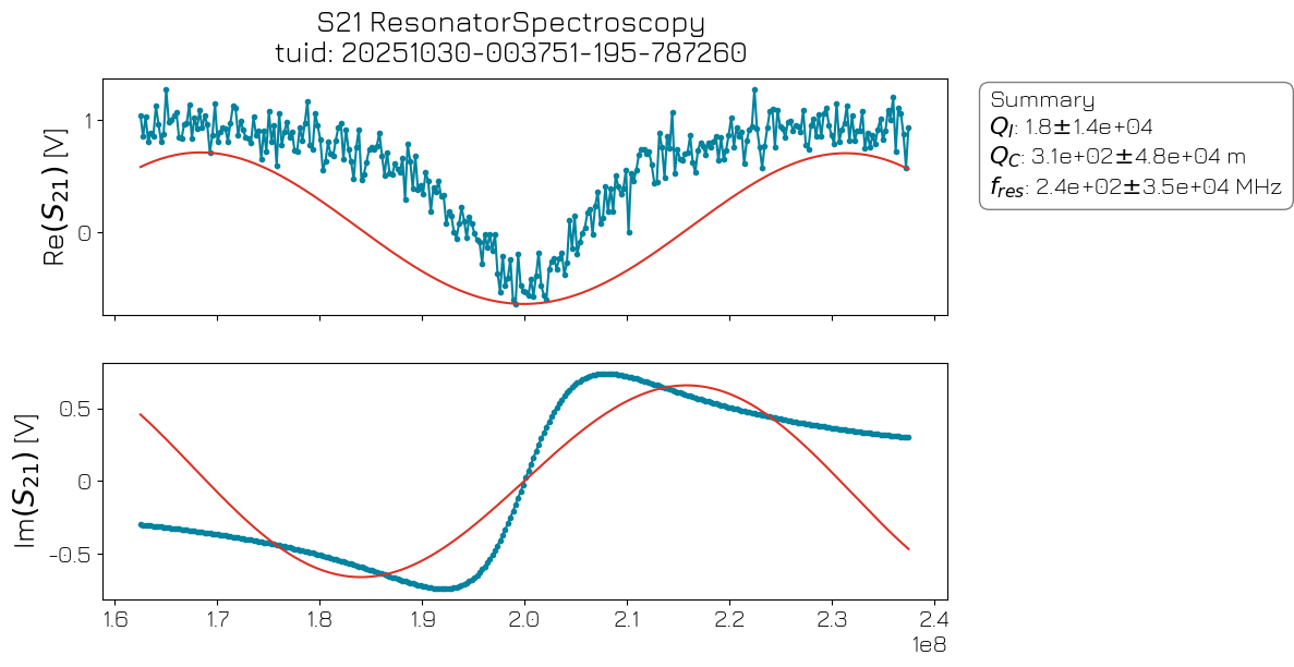
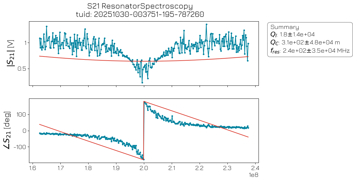
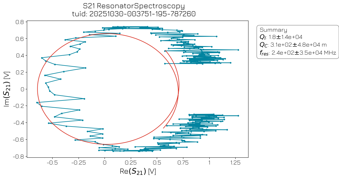
[11]:
res_spec_analysis = ResonatorSpectroscopyAnalysis(
    dataset=res_spec_data,
)  # settings_overwrite={"mpl_transparent_background": False}
res_spec_analysis.run().display_figs_mpl()
The quantum device settings can be saved after every experiment for allowing later reference into experiment settings.
[12]:
hw_agent.quantum_device.to_json_file("./dependencies/configs", add_timestamp=True)
[12]:
'./dependencies/configs/spin_with_psb_device_config_2026-02-04_00-27-53_UTC.json'