See also

A Jupyter notebook version of this tutorial can be downloaded here.

RF control

In this tutorial, we demonstrate control of RF modules over a large frequency range (\(2.0\) - \(18.0\) GHz) by sweeping the LO frequency;

To run this tutorial, you will need:

• QRM-RF

• An SMA-cable

Setup

First, we are going to import the required packages.

from __future__ import annotations

import json
from typing import TYPE_CHECKING

import matplotlib.pyplot as plt
import numpy as np
from qcodes.instrument import find_or_create_instrument

from qblox_instruments import Cluster, ClusterType

if TYPE_CHECKING:
    from numpy.typing import NDArray

Scan For Clusters

We scan for the available devices connected via ethernet using the Plug & Play functionality of the Qblox Instruments package (see Plug & Play for more info).

!qblox-pnp list

cluster_ip = "10.10.200.42"
cluster_name = "cluster0"

Connect to Cluster

We now make a connection with the Cluster.

cluster: Cluster = find_or_create_instrument(
    Cluster,
    recreate=True,
    name=cluster_name,
    identifier=cluster_ip,
    dummy_cfg=(
        {
            2: ClusterType.CLUSTER_QCM,
            4: ClusterType.CLUSTER_QRM,
            6: ClusterType.CLUSTER_QCM_RF,
            8: ClusterType.CLUSTER_QRM_RF,
            10: ClusterType.CLUSTER_QTM,
            12: ClusterType.CLUSTER_QRC,
        }
        if cluster_ip is None
        else None
    ),
)

cluster.reset()
print(cluster.get_system_status())

Status: OKAY, Flags: NONE, Slot flags: NONE

Get connected modules

# QRM-RF modules
modules = cluster.get_connected_modules(lambda mod: mod.is_qrm_type and mod.is_rf_type)
# This uses the module of the correct type with the lowest slot index
module = list(modules.values())[0]

Spectroscopy Measurements

A common experimental step is to find the resonance frequency of a resonator. To showcase the experience flow in this case we will sweep close to the full frequency range of the QRM-RF module (\(2\) - \(18\) GHz) and plot the frequency response.

We start by defining a function to plot the amplitude and phase of the output signal.

def plot_spectrum(freq_sweep_range: NDArray, I_data: NDArray, Q_data: NDArray) -> None:
    amplitude = np.sqrt(I_data**2 + Q_data**2)
    phase = np.arctan2(Q_data, I_data) * 180 / np.pi

    fig, [ax1, ax2] = plt.subplots(2, 1, sharex=True, figsize=(15, 7))

    ax1.plot(freq_sweep_range / 1e9, amplitude, linewidth=2)
    ax1.set_ylabel("Amplitude (V)")

    ax2.plot(freq_sweep_range / 1e9, phase, linewidth=2)
    ax2.set_ylabel(r"Phase ($\circ$)")
    ax2.set_xlabel("Frequency (GHz)")
    fig.tight_layout()
    plt.show()

Setup

Connect the output \(\text{O}^{1}\) of the module to input \(\text{I}^{1}\).

Initially, we need to define the acquisition memory. As we are using the NCO and a DC offset to generate an IF signal, so we do not need a waveform. We need to make sure that the acquisition is delayed relative to the output to compensate for the time of flight (the acquisition_delay). Finally, we will also add averaging to increase the signal-to-noise ratio (SNR) of the measurements.

# Parameters
no_averages = 10
integration_length = 1024
acquisition_delay = 200

For simplicity, a single bin is used in this tutorial.

# Acquisitions
acquisitions = {"acq": {"num_bins": 1, "index": 0}}

Now that the waveform and acquisition have been specified for the sequence, we need a Q1ASM program that sequences the waveforms and triggers the acquisitions. This program plays a DC wave, waits for the specified hold-off time and then acquires the signal. This process is repeated for the specified number of averages, with the average being done within the hardware.

seq_prog = f"""
      move    {no_averages},R0           # Average iterator.
      reset_ph
      set_awg_offs 10000, 10000          # set amplitude of signal
loop:
      wait     {acquisition_delay}          # Wait time of flight
      acquire  0,0,{integration_length}  # Acquire data and store them in bin_n0 of acq_index.
      loop     R0,@loop                  # Run until number of average iterations is done.
      stop                               # Stop the sequencer
      """

# Add sequence to single dictionary and write to JSON file.
sequence = {
    "waveforms": {},
    "weights": {},
    "acquisitions": acquisitions,
    "program": seq_prog,
}
with open("sequence.json", "w", encoding="utf-8") as file:
    json.dump(sequence, file, indent=4)
    file.close()

# Upload sequence
module.sequencer0.sequence("sequence.json")

In the RF modules, there is a switch directly before the output connector, which needs to be turned on to get a signal out of the device. The switch is controlled through the marker interface, first we must enable to override of the marker, then we must set the appropriate bits to enable the signal at the output.

module.disconnect_outputs()
module.disconnect_inputs()

# Enable marker switches to toggle the RF switch before output port
module.sequencer0.marker_ovr_en(True)
module.sequencer0.marker_ovr_value(3)

module.sequencer0.connect_sequencer("io0")
module.sequencer0.mod_en_awg(True)
module.sequencer0.demod_en_acq(True)

module.sequencer0.nco_prop_delay_comp_en(True)

module.out0_in0_lo_freq(3e9)
module.sequencer0.nco_freq(10e6)

# Configure the sequencer
module.sequencer0.integration_length_acq(integration_length)

# NCO delay compensation
module.sequencer0.nco_prop_delay_comp_en(True)

Now we are ready to start the spectroscopy measurements.

freq_range = np.arange(2e9, 18e9, 0.1e9)
lo_data_0 = []
lo_data_1 = []

for freq in freq_range:
    # Update the LO frequency.
    module.out0_in0_lo_freq(freq)

    # Clear acquisitions
    module.sequencer0.delete_acquisition_data("acq")

    module.arm_sequencer(0)
    module.start_sequencer()

    # Wait for the sequencer to stop with a timeout period of one minute.
    module.get_acquisition_status(0, timeout=1)

    # Get acquisition list from instrument.
    data = module.get_acquisitions(0)["acq"]

    # Store the acquisition data.
    lo_data_0.append(data["acquisition"]["bins"]["integration"]["path0"][0])
    lo_data_1.append(data["acquisition"]["bins"]["integration"]["path1"][0])

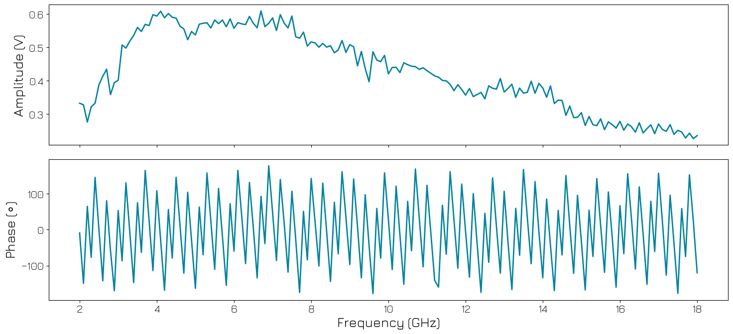
We plot the acquired signal’s amplitude and phase.

# The result still needs to be divided by the integration length to make sure
# the units are correct.
lo_data_0 = np.asarray(lo_data_0) / integration_length
lo_data_1 = np.asarray(lo_data_1) / integration_length

# Plot amplitude/phase results
plot_spectrum(freq_range, lo_data_0, lo_data_1)

Stop

Finally, let’s stop the sequencers if they haven’t already and close the instrument connection. One can also display a detailed snapshot containing the instrument parameters before closing the connection by uncommenting the corresponding lines.

# Stop all sequencers.
module.stop_sequencer()

# Print status of sequencers 0 and 1 (should now say it is stopped).
print(module.get_sequencer_status(0))
print(module.get_sequencer_status(1))
print()

Status: OKAY, State: STOPPED, Info Flags: FORCED_STOP, ACQ_SCOPE_DONE_PATH_0, ACQ_SCOPE_DONE_PATH_1, ACQ_BINNING_DONE, Warning Flags: NONE, Error Flags: NONE, Log: []
Status: OKAY, State: STOPPED, Info Flags: NONE, Warning Flags: NONE, Error Flags: NONE, Log: []