

User Guide for qblox-scheduler#
Get started with qblox-scheduler by exploring the essentials:
Control Flow: Learn how to create complex pulse- and gate-level schedules.
Hardware Configuration: Configure your Qblox modules directly through the scheduler.
Core Concepts: Dive into the underlying mechanics to understand the scheduler’s nuances.
Core concepts#
Experiments in qblox-scheduler run sequences of pulses and acquisitions, returning the results in a
xarray.Dataset structure.
On the user side, the package introduces these core concepts:
The
HardwareAgentclass
In this document, we shall present the HardwareAgent class, which is the fundamental interface
between users and the hardware backend of the Qblox control stack. We will also present the different types of data
returned by the execution of experimental sequences, these sequences are named Schedules in the qblox-scheduler
framework.
Each of the other core concepts listed above has its own dedicated documentation page, which we encourage the interested reader to explore for more detail.
The HardwareAgent class#
Generalities#
The HardwareAgent class is the primary interface for controlling a Qblox-based experimental
setup. It provides a software representation of the hardware stack, including the quantum hardware as well as the qblox
clusters and modules.
Its main responsibilities are to:
Describe the hardware setup: it loads the physical layout and static settings for the instruments.
Manage experiment execution: it serves as the main interface for compiling and running experiments on the hardware and retrieving the resulting measurement data.
The HardwareAgent is configured using two configuration files:
the hardware configuration: a required file that defines the hardware components (clusters, modules) and their instrument settings.
device configuration: an optional file describing the device under test (DUT) and the logical operations that can be performed on it. In the context of quantum computing, that DUT will often be a quantum processing unit (QPU).
To get started, you instantiate the HardwareAgent with these configuration files:
hw_agent = HardwareAgent(hardware_configuration, quantum_device_configuration)
Configuration files#
Detailed documentation for the hardware configuration and the device element configuration can be found on their respective pages.
Hardware configuration and pulse-level schedules#
In a minimal setup, only the hardware configuration is required. Providing it to the
HardwareAgent enables the description of an experimental sequence in terms of pulses and
acquisition operations, without introducing the notion of device under test and gates.
You can provide the hardware configuration to the HardwareAgent in one of three ways:
As a Python dict.
As a JSON or YAML file representing that dictionary.
As a
QbloxHardwareCompilationConfiginstance.
Example of a hardware configuration dictionary
hardware_config = {
    "version": "0.2",
    "config_type": "QbloxHardwareCompilationConfig",
    "hardware_description": {
        "cluster0": {
            "instrument_type": "Cluster",
            "modules": {
                "2": {"instrument_type": "QCM"},
                "4": {"instrument_type": "QRM"},
                "6": {"instrument_type": "QCM_RF"},
                "8": {"instrument_type": "QRM_RF"},
                "10": {"instrument_type": "QTM"},
            },
            "ref": "internal",
            "ip": "<cluster_IPv4>",
        }
    },
    "hardware_options": {},
    "connectivity": {
        "graph": [
            ["cluster0.module4.complex_output_0", "q0:port"],
            ["cluster0.module4.complex_input_0", "q0:port"],
        ]
    },
}
For more complex examples, please refer to the hardware configuration page. With a valid hardware
configuration, the HardwareAgent understands which modules are available and which ports can
be targeted by operations. This allows for the direct compilation and execution of pulse-level schedules, as shown
below:
Pulse-level schedule example
# Create a schedule
# -----------------
schedule = Schedule("Minimal pulse-level schedule")

# Play a 1 µs square pulse with an amplitude of 0.577_215 on "q0:port".
schedule.add(
    SquarePulse(
        duration=1e-6  # duration of the square pulse is 1 us.
        amplitude=0.5  # amplitude of the square pulse is 0.5 of the full scale.
        port="q0:port" # string used to search in connectivity graph for the actual output port.
        )
)

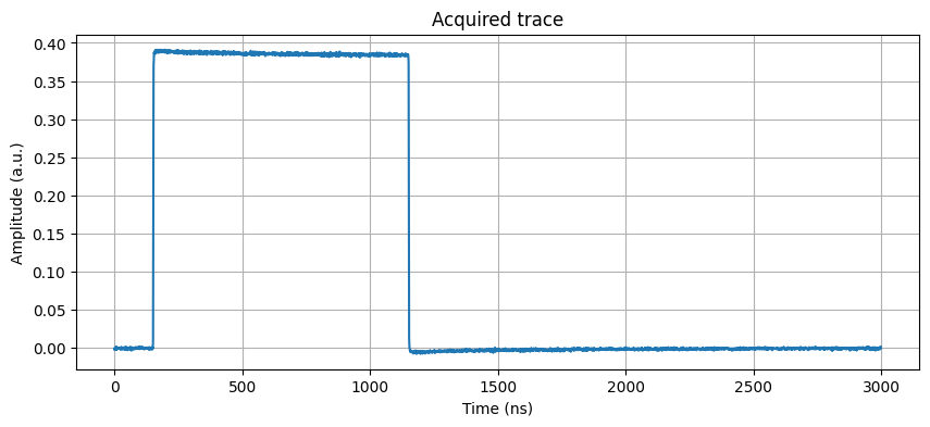
# Simultaneously, start a 3 µs trace acquisition on the same port.
# A Trace acquisition captures a waveform, similar to an oscilloscope.
schedule.add(
    Trace(duration=3e-6, port="q0:port", clock="cl0.baseband"),
    ref_pt="start",
)

# Execute the schedule
# --------------------
xr_trace_acquisition = hardware_agent.run(schedule)
Executing this schedule returns the following trace acquisition data:
Device element configuration and gate-level representation of a schedule#
Optionally, you can provide a device configuration to enable a gate-level description of your experiment. This file defines a collection of elements (like qubits) and their associated logical operations (gates). Each gate corresponds to a pre-defined sequence of pulses and acquisitions. Using this higher-level of abstraction simplifies the process of writing complex quantum algorithms by abstracting away the underlying pulse details.
Example of device element configuration
device_config = {
    "name": "qpu_0",
    "elements": {
        "qubit_0": {
            "name": "q0",
            "element_type": "BasicTransmonElement",
            "reset": {
                "name": "reset",
                "duration": 100e-6,
            },
            "rxy": {
                "name": "rxy",
                "duration": 40e-9,
                "amp180": 0.1,
                "beta": 0.0,
            },
            "measure": {
                "name": "measure",
                "pulse_type": "SquarePulse",
                "pulse_duration": 5e-06,
                "pulse_amp": 0.05,
                "acq_label": 0,
                "acq_delay": 200e-09,
                "integration_time": 5e-06,
                "reset_clock_phase": True,
                "acq_weights_a": {"data": "", "shape": [0], "dtype": "float64"},
                "acq_weights_b": {"data": "", "shape": [0], "dtype": "float64"},
                "acq_weights_sampling_rate": 1.0,
                "acq_weight_type": "IQIntegration",
                "acq_rotation": 0,
                "acq_threshold": 0,
            },
            "ports": {
                "name": "ports",
                "microwave": "q0:mw",
                "flux": "q0:fl",
                "readout": "q0:res",
            },
            "clock_freqs": {
                "name": "clock_freqs",
                "f01": 4.349_984_473e9,
                "f12": 0,
                "readout": 7.393_717_793e9,
            },
        },
    },
}
In this example, the BasicTransmonElement implements \(\hat{R}_{xy}\) gates using DRAG pulses, with the
modulation frequency taken from the clock_freqs.f01 entry, and a measure gate using a square pulse. For more information about what “ports” and “clocks” mean, please check this tutorial page. Note that after qblox-scheduler V1.0, BasicTransmonElement needs to be imported from qblox-applications.
This dictionary describes a single-qubit QPU that supports Reset, Measure, and rotation operations
(\(\hat{R}_{xy} (\theta, \phi)\)). By defining the static parameters for these gates, the
HardwareAgent can transpile them into the correct pulse sequences. The available and required
fields of this configuration are depending on the qubit architecture, and therefore the subsequent implemented
element_type class. Below figure illustrates the general structure of the qblox-scheduler user-side concepts, and
the way they interconnect.

General structure of the qblox-scheduler user-side concepts, and the way they
interconnect.#
Dataset#
Generalities#
The execution of schedules by an instance of HardwareAgent is ensured by the
HardwareAgent.run method, which returns a xarray.Dataset
(xarray documentation).
More details about the structure of those datasets can be found in the
acquisitions tutorial page of qblox-scheduler. The important
idea is that the acquired data are stored in a “Data variables” mapping under the form of xarray.DataArrays, and the
values of those data series are indexed with “Coordinates” (typically a set of experimental parameters that was applied
when the data point was taken). An example of such a dataset is given below, where the xarray.DataArray “data” has
values depending on the (frequency, amplitude) coordinate system.
<xarray.Dataset> Size: 48kB
Dimensions:               (acq_index_data: 1000)
Coordinates:
  * acq_index_data        (acq_index_data) int64 8kB 0 1 2 3 ... 996 997 998 999
    amplitude             (acq_index_data) float64 8kB -1.0 -1.0 ... 1.0 1.0
    frequency             (acq_index_data) float64 8kB 8e+07 ... 8.25e+07
Data variables:
    data                  (acq_index_data) complex128 16kB (-0.05443004396678...
Attributes:
    tuid:     20250911-164958-178-63babd
By default, the acquired data are assumed to be potentially sparse, meaning that they do not densily populate the grid
of available parameters listed in the Coordinate section: in practice the data and coordinate series are one
dimensional, and all indexed by the acq_index_<acq_label> array of integers (or trace_index_<acq_label> array for
Trace acquisitions). Nevertheless, this representation can be changed with the acq_coords_to_dims that can be loaded
from the qblox_applications.qblox_scheduler.analysis.helpers module, so that the acquired data becomes
multi-dimensional with physical coordinates (e.g. frequency and amplitude) being its dimensions. This can facilitate
further data analysis and visualization. An example is provided in the dedicated
acquisitions tutorial.
Data saving#
One can also notice the presence of a time-based unique id (tuid) attached to datasets. This tuid simplifies the
retrieval of data saved on a filesystem. Indeed, by default data are saved by the HardwareAgent in the
$HOME/qblox-data/<YYYYMMDD>/<tuid>/ directory, where $HOME is /home/username on Linux, /Users/username on macOS,
and C:\Users\username on Windows.
xarray.Datasetare saved in a HDF5 formatted file, with default namedataset.hdf5.The saving of data can be deactivated when the
HardwareAgent.runmethod is called: using thesave_to_experiment=Falseoptional argument.The default data directory can be overridden at the HardwareAgent instantiation, using the
output_diroptional argument.Loading datasets from hard drive is made easy with the
ExperimentDataContainerthat can be loaded withfrom qblox_scheduler import ExperimentDataContainer
this class implements many
classmethodsdesigned to facilitate data handling. The interested user can refer to the API documentation for an exhaustive description of thedata_handlingmodule ofqblox-scheduler, but just to name a few:load_datasetenables loading data from theirtuid.load_dataset_from_pathdoes the same but providing a path rather than thetuid.get_latest_tuidreturns the most recenttuid.
Saving Hardware Snapshots#
In addition to the raw data saved in datasets, qblox-scheduler also features the saving of low-level hardware
description and configuration. This functionality is inherited from the QCoDeS data acquisition framework, and
is documented here. These
snapshot collecting information about the instruments in use, are saved by default in the same directory as the dataset
files ($HOME/qblox-data/<YYYYMMDD>/<tuid>/), in a snapshot.json JSON file.
To summarize the different ways of saving measurement data and hardware snapshots using
HardwareAgent.run(..., save_to_experiment=..., save_snapshot=...): save_to_experiment = True, it saves measurement
data to disk; save_snapshot = True, it saves hardware snapshots to disk. Users can decide which combinations to use to
either save measurement data or hardware snapshots, or both.